CDT 档案卡
标题:毒死小狗获刑4年,Papi妈妈漫长的追凶
作者:阿尔莎发表日期:2025.12.10
来源:最人物主题归类:动物保护CDS收藏:公民馆版权说明:该作品版权归原作者所有。中国数字时代仅对原作进行存档,以对抗中国的网络审查。
详细版权说明。
2025年12月11日,在经历漫长的1184天后,“Papi妈妈”Penny终于等来了一个结果:
被告人张某华构成投放危险物质罪,被判处有期徒刑四年。张某华当庭提出上诉。
这天的北京低温零下2度,前一天的凌晨3点,睡不着的Penny在社交媒体上发:注定是个“输”,Papi回不来了,但希望能“赢”。
如今,她等来了这场“注定是输的赢”。
在过去的3年里,Penny的人生时钟几乎停摆,她不再考虑30岁后的就业危机,放弃工作,翻遍裁判文书网,查无可查后,决定自学刑法。网暴也从此刻,如影随形。
而这一切的起点,要回到2022年9月14日,抢救台上,一只小狗疑似中毒去世。几乎没人注意到它们。在一座住着2000万多万人口的大城市里,少有人在乎一只小狗的离开。
小狗叫Papi,是只步入老年的西高地白梗。他有双圆溜溜的眼睛,到离开时依旧努力睁得很大。如果当时平安走下手术台,几个月后就是它13岁的生日。
因为宠物殡仪下班,Penny把Papi抱回了家。小区楼下聚集着很多人,有人把手机怼到她面前,一边拍一边喊:“快看呀,北京朝阳区首开畅颐园小区投毒了,狗都死啦。”
那一天,小区内有11只宠物狗中毒,其中9只死亡,另有两只流浪猫死亡。
Papi回到了它的小床,盖好被子。Penny一夜不敢合眼,她的手一直在抖,内心却无比坚定,抓到凶手。
5个月后,她和小区受害犬抚养家庭组成了前所未有的11人起诉队伍。11只中毒犬,11份起诉书。
这成为北京甚至上广深等一线城市第一例走到刑事诉讼阶段的宠物中毒案。也在社会层面上,引发诸多关于“养犬行为”的讨论。
理性之外,质疑与网暴也层出不穷:连人的事情都管不过来,还要管狗的事情?
对此,Penny回应:“我想告诉大家,这从头到尾就是一个人的事情,我们一共有11位受害人,11个破碎的家庭。”
如今,Penny等来了一个结果,虽然被告当庭提出上诉,一切尚未结束,但在偌大的城市里,Penny终于为那些被毒死的小狗们,掀起了一点波澜。
那是哭声、惨叫声此起彼伏的一天,是Penny永远忘不掉的日子,2022年9月14日。
从小区附近的宠物医院,到几十公里外需要花费上万元血透的顺义宠物医院,都是同一个小区的居民和他们正在抢救的小狗。
十几只不满周岁的幼犬、怀孕的母犬和陪伴超过10年的老年犬,先后被送上抢救台。很多小狗前后15分钟就没了。
秋田犬“秋天”离开后,它的主人因痛哭缺氧,眼部剧痛被救护车带走,此后半年没能上班。
老年犬黄黄做完血液透析,不到十分钟便离开了。它是只流浪狗,两个月大时被现在的主人收养。互相陪伴的13年,老人为他做了被褥、枕头,一家人从未让黄黄在地上睡过觉。
现在,Penny眼看着黄黄被家人裹着医院给的小毯子抱走。黄黄家中的老人,因打击过大而住院。
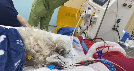
排在黄黄后面的是Papi。毒发后,它坚持了六个多小时,连抢救的宠物医生都惊叹于Papi的求生意志。
晚上六点多,血透结束。Papi开始抽搐,四肢奋力地划着,像溺水者努力想浮出水面。它又坚持了半个多小时。
Papi一直都很勇敢,从前打针都一声不吭,现在,它仍是年纪最大坚持最久的小狗。
可Penny还是收到了医院递来的毯子。
19:10,Papi不再抽搐,圆溜溜的眼睛却没闭上。Penny摸了摸手里的毯子,很廉价的质感,又哭了,她替Papi觉得委屈。
她从来都把能够到最好的一切给Papi。
Papi,在西班牙语里是好兄弟的意思。2010年,妈妈把两个月的小狗带到她身边,她为它取名Papi,把它当兄弟,再后来视作她的家人、孩子。
他们互相陪伴了12年,一起上山、看海、爬长城。Papi7岁步入中老年后,出行有了作为代步工具的小推车;查出高血脂和轻度的肾衰竭后,食谱新增了果蔬、鱼油和辅酶Q10,以控制体重。
Penny的分离焦虑一天比一天更重。每一天睡觉前,听着Papi微微的鼾声,她都在祈求时间再慢一点。每一年,Papi的检查费用比她自己的还高。
如今她的小狗走了,裹住它的怎么会是一条这么差的的毯子?
Penny又看了看Papi的病理报告单,上面写着:“肝脏指标升高,血钾过高,肌酸激酶升高,高度疑似中毒”。
这和Penny的猜想吻合,她猜到这明显无疑的非自然死亡,极大可能是有人投毒。
当天早上八点,她例行带Papi出门散步。十点,她收到小区朋友迟来的提醒,小区已经死了三只小狗,疑似中毒。
两小时后,Papi开始呕吐、吐血,浑身抽搐,送医抢救。
Penny在半小时后赶到,并立刻拨打110。医生透露,上午已经送来十几只,医院救不过来了。
她将医生的嘱托转发到小区住户群里,“赶紧通知小区物业,不要再遛狗了,或者是戴上嘴套”。
连发三遍提醒后,立刻有个叔叔回应了Penny。这是Penny联系到的第一个中毒犬的主人。
下午,Penny将Papi转到几十公里外可以全身换血的医院后,又遇到了同小区的黄黄。
夜里,Papi以几乎是最残忍的方式离开了他。
怀里的Papi似乎重了很多,Penny手一直在抖,几乎抱不住它。它的脖子为了扎针插管,用棕色的弹力绷带缠了五六层,如今就像要断掉一样。
Penny把Papi放回了它的小床,盖好被子。
家已经不是家了,像是不可言说的犯罪现场,到处是Papi吐的血、呕吐物和失禁时的大小便。
Penny想起了过去快速划过的投毒新闻。
全国各地,毒杀犬只事件时有发生。内蒙古通辽市,8只宠物狗吃下掺有鼠药的熟鸡肝块死亡;黑龙江牡丹江市,11只宠物犬被投毒致死;四川成都、云南昆明,小区宠物狗接连被投毒致死,且发生了不止一次……
那时她总抱着侥幸心态,不敢细看。这一刻,看过的新闻,过去从事记者的经验让她意识到,这是故意投毒,且投毒者大概率就住在这个小区。
Penny掏出手机,快速联系警方进行尸检、联系殡仪。她的手一直在抖,内心却无比坚定,一定要把人揪出来。
想讨回公道的不止Penny。那一天,她当时所在的畅颐园小区共拨出了24个报警电话。
首开畅颐园小区只有三栋楼12个单元,一天里却有11只宠物狗疑似中毒,9只死亡。这在整个小区内引起了恐慌。
中毒犬的主人们拼凑信息后发现,有交集的地方离小区儿童游乐场只有半米远。许多孩子每天在此玩耍。
家长不敢再让3岁的孩子在楼下逗留,几个月的时间里,抱着孩子进出。
养宠物的人,出门把自家小狗牢牢抱在怀里。投喂流浪猫的阿姨发现,小区的流浪猫都消失了。
中毒事件后,楼下出现了很多走访调查的便衣警察,询问有没有看到谁跟谁有冲突之类的问题。Penny后来得知,朝阳重案组四个队全部出动了。
她也每天在小区里绕,绝口不提受害者的身份,找机会和所有人聊,终于从刑警口中得知小区里被投放的危险物质名为氟乙酸,剧毒,属国家明令禁用的化学品,不能在市场流通和售卖。
零点几毫克氟乙酸即可致成年人死亡,对于Papi这样的小型犬来说,闻嗅即可致命,哪怕戴好嘴套也不能幸免。
半个月后,65岁的男性业主张某某因涉嫌故意投放危险物质罪,被抓获归案。
张某某后来在法庭上交待,他在市集买了鸡脖子,将吃剩的鸡脖剁碎,浸泡在氟乙酸药水里,撒到人来人往的车棚门口和儿童乐园附近。下毒是因为孙女不喜欢小狗,且他的三轮车曾被狗撒尿。
但北京市六环路以内禁止正三轮摩托车通行,且据Penny所说,嫌疑人的车一直停在小区内阻碍消防通道的地方。与这些违规相对应的是,中毒的小狗都有狗证,办了正规手续。
派出所最初以“被故意损毁财物案”受理,确定是氟乙酸后,变更为寻衅滋事罪。法律是Penny的知识盲区,她想知道是否可以数罪并罚,却发现各方都讲不太清楚。
Penny又在新闻和裁判文书网里寻找可参考案例。大量检索后发现,北上广深宠物中毒的新闻,仅可以检索到警方立案,但都没有下文,裁判文书查无可查。
她联系身边的大V、咨询北京头部的刑事诉讼律师,自学走法律程序和搜集更多有利证据的方法。但更细节的问题,他们都无法给Penny一个答案。
最近许多网友发给她的黑龙江宠物中毒被判刑案件,她在事发时,就已经仔细研读过公开卷宗,两案有太多不同。
没人接触过这样的案子。这是一个发生在一线城市的,与杀人放火、诈骗……都无关的,由宠物中毒而立案的刑事附带民事诉讼。哪怕是置身动物保护领域的律师,答复依旧是:第一次经手这样的案子。
善恶有报,Penny想要投毒者坐牢。摆在面前的卷宗和答复却告诉她,此前宠物中毒事件被刑事立案的少之又少,多数投毒者并没有受到实际刑事处罚,多是取保或赔钱。
接下来的路并不好走。Penny没有犹豫地继续为Papi而战。
没有可参考答案,她可以耗上自己的人生来寻找、答题。
她买来《刑法》《民法典》《刑事诉讼法》《民事诉讼法》,从基本法看起,逐字逐句寻找适用的法条,将法律真正当作自卫的武器。
自学法律的同时,她还有件更重要的事,连接11人的起诉队伍。
中毒犬的主人陆陆续续进群。每个人都想为自己的小狗讨回公道,可其中有人上了年纪不知所措,有人忙于工作没有空闲时间,有人受制于经济压力。
她做好起诉状模板,一家一家去聊。其中50%是中老年人,个别打字、认字都受限制,他们嘱咐Penny:“闺女,你别给我打字儿,你给我发语音。”电话沟通成本非常高,解释时间以小时起步。
Penny把所有人当作工作的甲方,不断去调整要求,直到每一步大家都能达成共识。
事发一年后,最后一个中毒犬的抚养女孩进入中毒小狗的受害群。她不善社交,却实在放不下她的小狗,于是在小区群询问:“一年前的这个事情就这样结束不了了之了吗?”
Penny问女孩,要不要起诉,对方立刻回答:“要”。
11只中毒犬,11人组成起诉队伍。
2022年12月,Penny收到的立案告知书显示,朝阳分局以张某某“投放危险物质罪”正式立案。2023年1月,朝阳法院正式立案。Penny等11名受害人的起诉书也陆续提交。
这是北京第一例走到刑事诉讼阶段的宠物中毒案。
立案后,Penny终于有时间停下来,去趟医院了。
此前的四个月里,Penny的时间被超负荷排满,每时每刻都在崩坏边缘徘徊。
她的爸爸急需手术,住院又和退休前手续办理等时间冲突。2022年在小区进出都困难的情况下,她作为独生女,不得不独自据理力争,帮父亲协调退休问题的同时,3个月里接连为父亲安排好两次心脏手术。
工作也在继续。Penny当时是国内某头部影视公司的骨干员工,恰逢负责的项目杀青上线,出品人、演员到视频平台的负责人,无数人无数消息等着她处理。
Papi离开后,Penny没睡过一个好觉。她整夜失眠,心率加快,耳鸣、发抖。人生第一次,Penny为了能呼吸,在家里准备了许多氧气瓶。
靠着吃药,她才能在天亮前后,勉强睡一会。有时候,梦里的尖叫声会把她吵醒,睁开眼,却再也没有Papi能感受到她低落的情绪,把爪子搭在她身上。
在梦里,Papi从没出现过。
Papi离开的第一周,她瘦了10斤,之后暴食又胖20斤。睡不着觉的凌晨三五点,她控制不住地大量进食,直到需要吃胃药时才能停下,也不止一次地走上天台。
她并不怕高。20多岁时,她爱玩敢闯,蹦极、跳伞、飞机跳、大风天开快艇,潜水到十几米的海下。
她不惧怕挑战,从体制内跨界互联网影视行业,主持年会,举办沙龙做演讲人,采访名导、明星。
现在,她的人生却相对静止了。2023年1月底,Penny确诊重度抑郁症和焦虑症,决定放下手中所有工作。朋友们发来的关心的、安慰,她无力回复,许多信息至今停在2022年或2023年的某天。
把她拉下天台的是Papi。她记得Papi尸检后,腹部那条被潦草缝上的口子、勉强才能合上的眼睛和裹着它难以形容的黄色袋子;记得收到Papi骨灰那天另外到来的三个快递,全部与Papi有关,里面装着原本打算带它中秋去阿那亚看海的海魂衫和救生衣。
Penny走下天台,按下工作、生活和社交的暂停键,只有关乎Papi的进度在持续加载。
她在重度焦虑和抑郁中,克服生理本能,苦读刑法,动力只有一个,让投毒者依法量刑。
后来,在宠物中毒最常用也最重的故意投放危险物质罪之外,Penny在《刑法》里发现了投毒人的行为可能还触犯了第125条里的“非法制造、买卖、运输、储存危险物质罪”,若“非法买卖、运输、储存原粉、原液、制剂500克以上”或“造成公私财产损失20万元以上的”,属于125条里“情节严重”的,“处十年以上有期徒刑、无期徒刑或者死刑”。
2023年2月,11人递交起诉状,要求“判处被告人故意投放危险物质罪,寻衅滋事罪,损毁他人私有财产罪,数罪并罚”;要求赔偿11个起诉人抢救费和精神损失费等。
Penny不止一次打电话询问开庭时间,对方最开始说大概在2023年3月,4月,最终延后至10月。2023年10月26日,案件在朝阳区人民法院温榆河刑事法庭开庭。
11个起诉人,全部到场。此时,距离11只小狗中毒死亡已过去一年零一个月。
开庭时,书记员得知投毒案是个狗的案子,一时没反应过来,“在法院待这么长时间,第一次听到狗中毒的事情还能走到刑事案件,没听说过。”
庭审现场,犯罪嫌疑人无悔罪表现,坚决拒绝所有赔偿。过去一年多,他和他的家属也从未对小区居民表达任何歉意。
宠物主中,上了年纪的大爷大妈第一次看到被告,控制不住情绪,在发言时已哭作一团。Penny看到,对方律师笑了笑,好像浑不在意。
Penny作为原告代表发言,坐在了公诉人旁边,成为除法警外,离被告最近的人。她也是原告席最冷静的一个。
因为法官的锤子已经敲了无数次。她不敢回忆,不敢落泪,强制自己跳出受害人角色,去安抚他人。她必须像正常人一样,才能去提问,才能不剥夺发言甚至旁听的资格。
中场休息时,对方律师告诉Penny:“我觉得你就应该当律师。你不考司法,太可惜了。”
法院的工作人员则告诉她,“以你的性格,我觉得你一定可以成的。”
可Penny翻阅卷宗、自学刑法以及她的冷静、口才,并没有等来一个结果。
下午四点,走出法庭,Penny发现,大门外,大家也都在等结果。
那天清早,许多人从全国各地赶来,得知庭审没有任何旁听席位,就守在门口。法院门前连把椅子都没有,公路上只有野狗在三两成群地散步,可他们在北京10月末的大风里,没有吃饭,一直站到了现在。
Penny的眼泪瞬间落下了。
案件并未当庭判决。
被告的实际量刑,要根据其是否造成严重后果,即“致人重伤、死亡或者使公私财产遭受重大损失的”。因目前该案未造成人员伤亡,是否造成公私财产遭受重大损失,要考虑鉴定价格和因投毒产生的就医费用。
这正是难点,11只受害犬的司法鉴定价格至今没做成功。因为所有小狗没有血统证,司法鉴定失败的理由写着:缺少鉴定参数。
Penny打电话给北京相关鉴定部门,对方的反应是,“从来没有听说过还有人给狗做鉴定的。”
抚养人们精心照顾的小狗,每年营养品价格上万,抢救费用上万,只因它不是名车、字画、古董文玩,所以哪怕Penny四处争取了两年,小狗们的价格依旧无法鉴定,无法证明。
11个人依旧在为所有人“没听说过”的案子坚持。一审后,他们决定请个律师,不再这么被动。
找律师、确定、签字,也是Penny带着律师一家一家去聊的。为此,她必须重返案发小区。
Papi离开后,她一夜夜睡在朋友的车里,搬家恰逢司机和保洁感冒都不能来,她宁愿和朋友来来回回搬了20多趟,也不愿在那待一天。
重回故地,Penny又想起了Papi。
世面见多了,Papi早早学会了享受狗生。在公园散步时,它会把脚搭在塑胶跑道上面,而不是兴奋地扑进草坪撒欢。它已经能清楚分辨水泥地、草坪和跑道哪个脚感更好,夏天草里是否打过药水。
小区里,很多人养了新的小狗,依旧是原来的品种,用着原来的名字。没人能彻底从伤痛中走出来。
而Penny无法再拥有一只小狗了。Papi就是她生命的一部分,她无法承受类似悲剧再来一次的风险。
“我总说没有人能共情我做的事。你把它想象成一个 13岁的小男孩,疼痛、抽搐、惊惧、尖叫、吐血、大小便失禁,整整将近 10 个小时,或许你才能共情我的痛苦。”
Papi离开的日子里,投毒者被关在看守所 ,Penny也被迫一起关着。
没人限制她的自由,她手脚的无形枷锁是她亲手戴上的。她不敢出门,活动范围限定在一日能往返的京津冀。判决书可能在任何一个工作日给到,如果结果不能接受,她必须在3个工作日内递交准备好的抗诉材料,且快递只能走中国邮政。如果人在异地,根本来不及。
而且出去去干嘛呢?近几年,她偶尔出门,在山里哭,在海边哭,在前往目的地的高铁上哭。
身边的朋友劝Penny,即便对方判4年,你都已经赢了100% 的养宠人。目前宠物刑事案件最重判刑3年7个月。
Penny不想要这样的胜利。她的诉求始终如一,清清楚楚明明白白查清案子。
抢救台上,Papi坚持了最长的时间。Penny则押注了更长的人生,既然有法可依,那当然得求个公道,讨个公平正义。
在此之前,她的生命卡在这里无限循环,她的名字只剩下一个,西高地Papi妈妈。
网暴从Penny为Papi讨公道的第一天就开始了。她给小狗讨公道,因此自然而然地成为了一部分人的“靶子”。
她在直播时回忆起最后一次抱着Papi的场景,哽咽着苦笑,被人骂怎么笑得这么开心;她半夜哭到控制不住,被人骂哭着作秀。哭笑说话都是错。
时间久了,Penny可以根据谩骂内容,判断网暴者性别。一方攻击的点是恶犬伤人、不文明养犬。另一方骂人的每一个字眼都是只跟女性相关的器官和疾病,且在男性身上并不通用。
上个月,她的私人信息被发在人肉爆料群,她发现后立刻去派出所报案,执法者觉得不可置信:“你确定吗?你不认识他?你确定你跟他无冤无仇没有见过吗?你们是素不相识的这种陌生人吗?”
答案是素不相识,无冤无仇。网暴的男人发现Penny真的去警局报案后,立马把她拉黑,并更换了头像封面。
也有来自求助者的道德绑架。
最初,只要有人求助,Penny半夜两点也会给出私人手机号,彻夜长聊。但他们总是很快就没了消息,偶尔还有人在一段时间后拉黑Penny。
她渐渐明白,有些询问者不是想讨回公道,而是想让她帮忙权衡利弊。
心力实在有限,Penny决定只为Papi发声,如果帮人发声,对方至少得先坚持300天。
于是她又被指责作为小狗英雄,凭什么不帮忙?而在Penny看来,她不是什么英雄,没有神通,只是个自身难保的泥菩萨。
何况,她坚持1000多天了,至今还没有一个坚持300天以上的人来找过她。
这是Penny碰到坏人最多的两年,也是碰到好人最多的两年。
有人想给她众筹,询问捐款通道,私信发口令红包。这些她从来都没收过。
有人为她提供未来工作的机会:“事情结束后,不嫌我们庙小,可以来工作。”这样的邀请,Penny已经收到了很多个。
常有陌生人发来上千字的安慰。每个人都告诉她,Papi只是结束了狗生,它会像一阵风,一道光或是以各种各样的方式回来,和你重逢。
安慰不是良药,Penny只想要坏人受到应有的惩罚。
不久前,Penny将她的经历授权给了一个影视公司。还有一个团队想把它孵化成话剧。她有时会想象,如果电影能拍出来,上映那天,会不会就是投毒者刑满释放的时候?
开剧本会时,她发自内心地羡慕着主创团队。过去身处影视行业,她偶尔抱怨工作生活始终分不开。真正丧失生活两年后,她才意识到,那时再卷再累,身边都是能正常沟通的人,进度总是在向前推进,那才是正常的工作和人生。
不像现在,yes or no的选项里,她得到的答复永远是or。
Penny并不享受Papi带来的流量,也不想面对媒体一次次挖开血肉。但只有表达,才能让更多人看到,让Papi被注意到。
鲁迅说,世界上本没有路,走的人多了,便成了路。
Penny也这么想。20年来养宠物的人从少到多,才有了这么多冻干零食和宠物友好的商场、交通,为小狗伸张正义的刑事诉讼也是一样。过去没有,现在很少,但她不是正在坚持吗?
Penny很喜欢《三大队》的主题曲《人间道》,歌里唱着:
“恶人还需犟人磨
我是你杀生得来的报啊
也是你重生的因果
为一口气 为一个理
为一场祭 老子走到底
……
我要白日见云霞夜里举火把
我要这朗朗乾坤下事事有王法”
Penny自认是个犟人,但不是向来如此。过去,她不是刚烈的性格,近几年的坚持,让她看到不合理的事,会主动站出来。
通过学到的刑法知识,她阻止过马戏团的动物表演,也成功举报过非法的狗肉产业链。“当你真正掌握了相关的法律法规,你会发现它真的很好用。”
她的《刑法》已经被翻到翘边。她发现,《刑法》是本太好用的书,对于大多数人来说,现行的法律法条就够用。
后来,有关注Papi案子进展的孩子妈妈真的买回了法律书籍,每天睡前陪着女儿读一章,希望孩子在未来遇到麻烦时,有能力用法律自保,而不是说一句“算了”。
能多影响一个孩子,Penny觉得太过于难得。她也想往前走,放手的前提还是那句话,坏人要得到惩罚。
近几年,她非必要不出门,已经很久没有好好化过妆,拍拍照,放松地过一天了。我们约在一个晴朗的的秋日。
微风吹过,她独自站在三里屯的街区,看着蓝天白云绿树,忽然有种特别抽离的感觉。
这是闹市的中心,是她曾经熟悉的地方,有着生活原本的模样。
*原文发布于 2024 年10月,今日重发,有删改。