As with other popular religious narratives, the nineteenth century brought innovation in the depiction of the Annunciation by the angel Gabriel to Mary, telling her that she will become the mother of Jesus Christ, the first step leading to the Nativity that follows in the coming week.
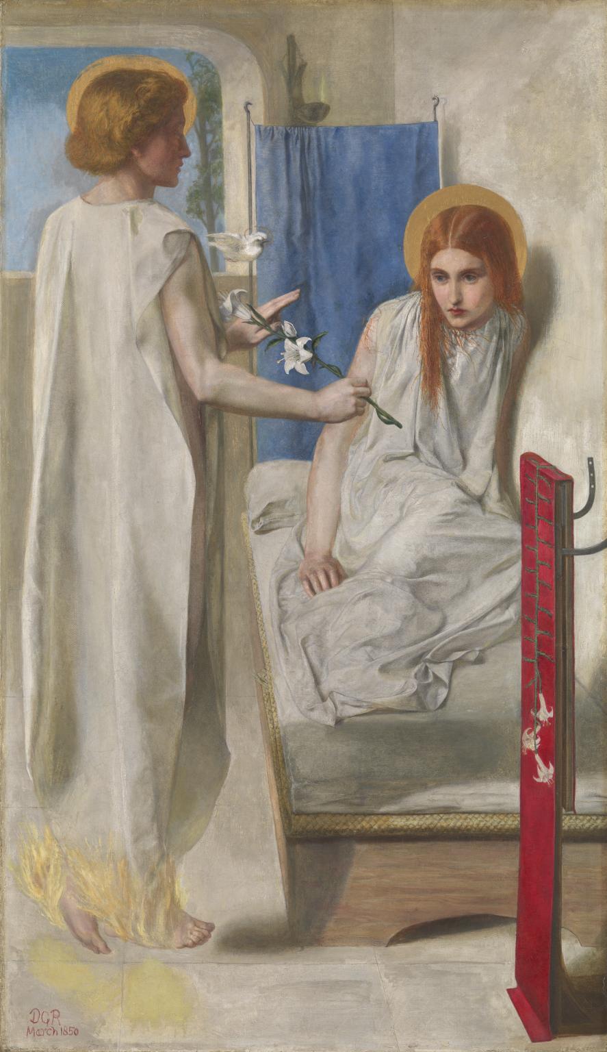
Dante Gabriel Rossetti’s Ecce Ancilla Domini! (The Annunciation) (1849–50) is as radical a reinterpretation of the traditional Annunciation painting, as his The Girlhood of Mary Virgin (1848-49) was of the life of Mary. There are gilt halos amid natural and realistic depictions of the figures and objects, in accordance with the ideals of the Pre-Raphaelite Brotherhood.
Symbols shown include: white robes for purity, the lily for purity and its traditional association with the Annunciation, a dove representing the Holy Spirit, red embroidery referring forward to Christ’s crucifixion, a blue curtain for heaven, and flames at the feet of the angel Gabriel rather than traditional wings.
Henry Ossawa Tanner (1859–1937), The Annunciation (1898), oil on canvas, 144.9 x 181.1 cm, Philadelphia Museum of Art, Philadelphia, PA. Wikimedia Commons.
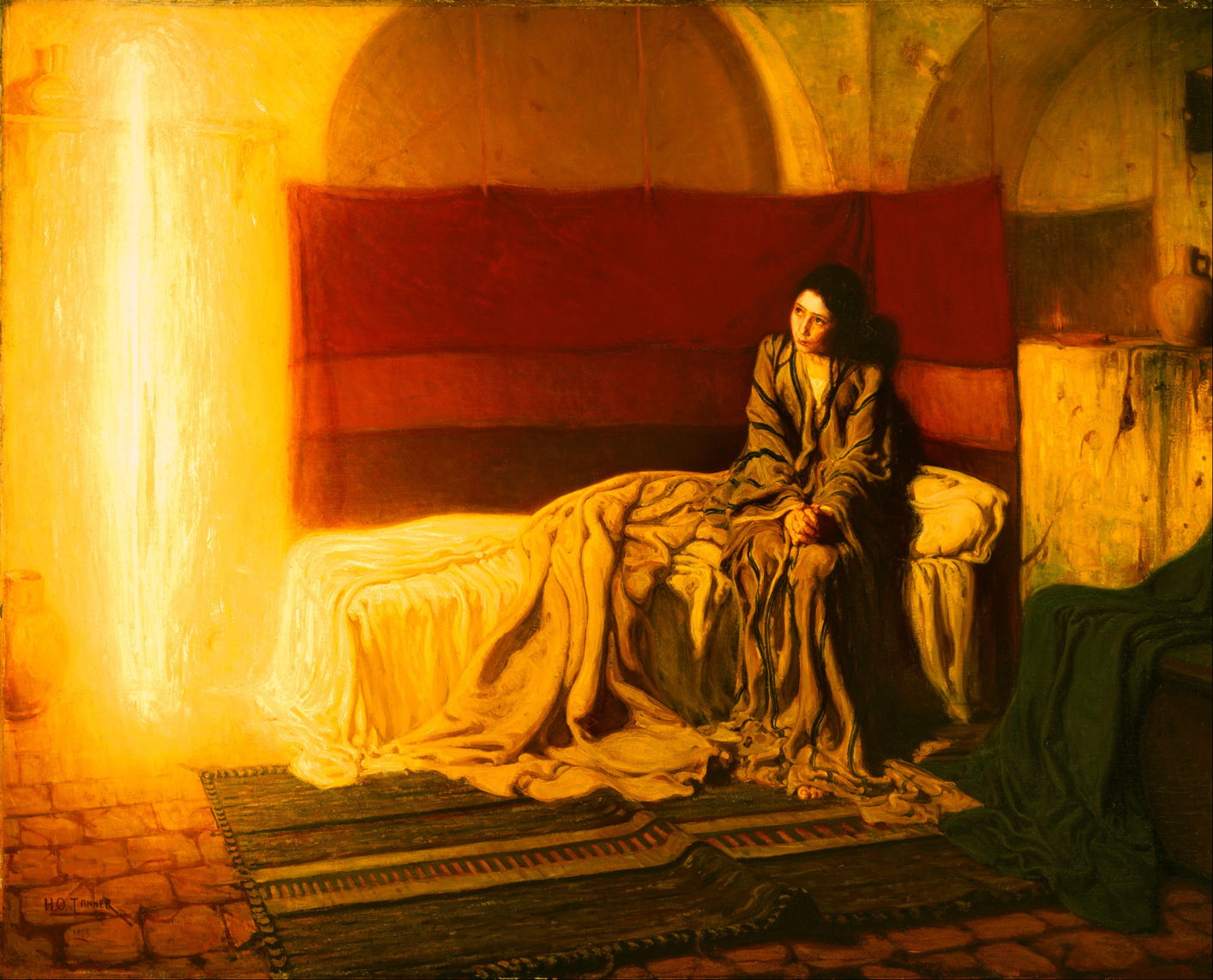
This Annunciation from 1898 is one of Henry Ossawa Tanner’s most unconventional paintings of a traditional scene. He sets it in the private space of Mary’s bedroom, with the bedclothes rumpled untidily, and Mary in casual night dress. There is no angel as such, but a dazzling fire of the spirit, forming a subtle crucifix with a shelf behind. This painting was accepted for the Salon of 1898, and was widely reproduced in magazines afterwards.
Vittorio Matteo Corcos (1859–1933), Annunciation (1904), oil on canvas, 220 x 180 cm, Convento di San Francesco, Fiesole, Italy. Wikimedia Commons.
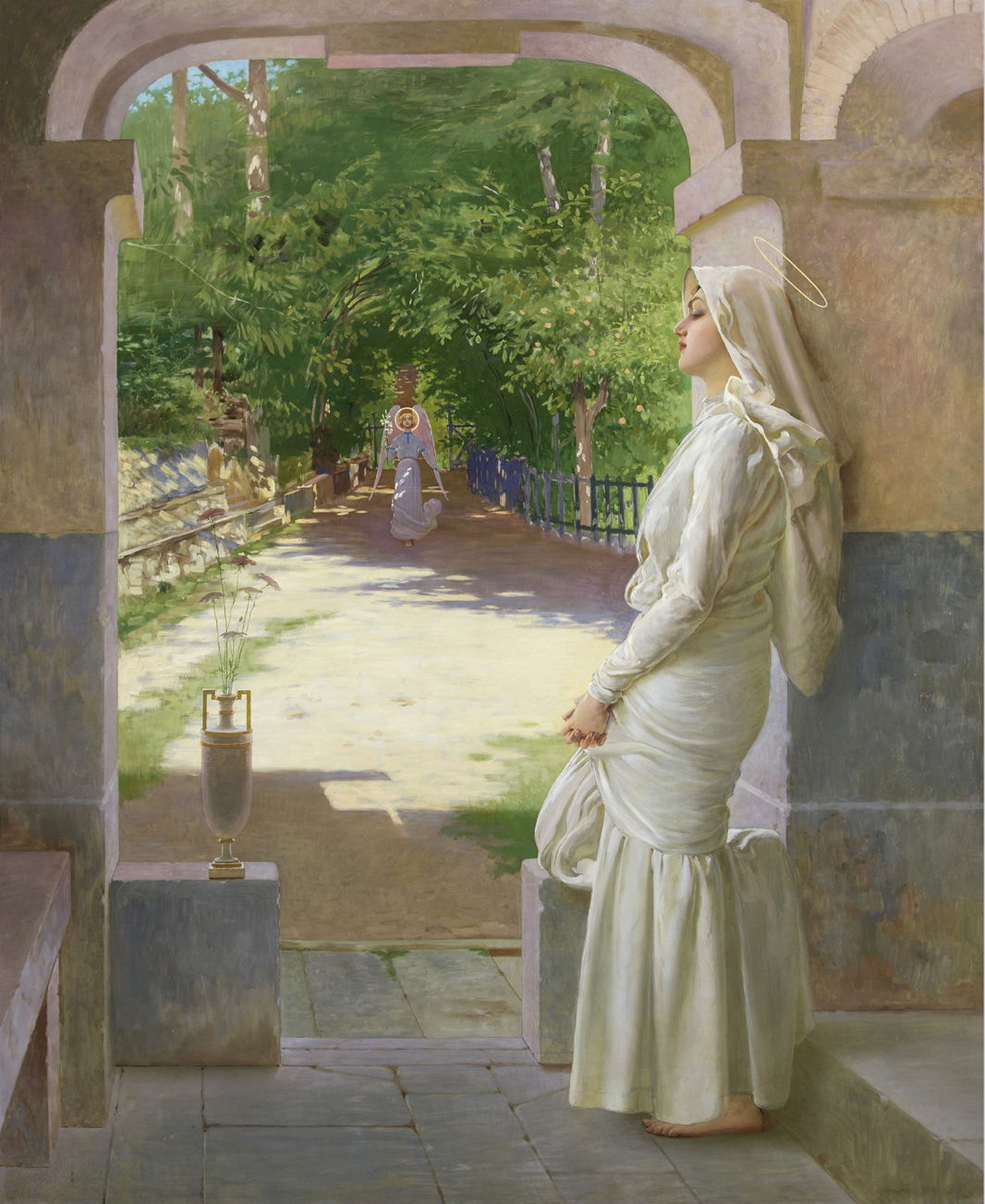
In 1904, Vittorio Matteo Corcos completed this remarkable painting for the Convento di San Francesco in Fiesole, Italy. Mary has a highly contemporary look as she stands in contemplation with her hands clasped together in prayer. Gabriel approaches from the distance, walking through a tunnel formed by trees.
Oleksandr Murashko (1875–1919), Annunciation (1907-08), oil on canvas, 198 x 169 cm, National Art Museum of Ukraine Національний художній музей України, Kyiv, Ukraine. Wikimedia Commons.
Of all these paintings, it’s Oleksandr Murashko’s Annunciation, probably from 1907-08 or 1909, that I find most breathtaking. Apparently, he was first inspired to paint this when he saw a girl part light curtains to enter his house from the terrace outside. He saw a parallel with the entry of the Archangel Gabriel in the Annunciation.
John William Waterhouse (1849–1917), The Annunciation (1914), oil on canvas, 99 × 135 cm, Private collection. Wikimedia Commons.
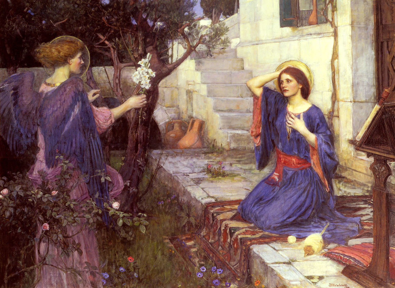
Just before the First World War broke out, John William Waterhouse painted his one and only religious work, The Annunciation (1914). Although completed over fifteen years after Tanner’s, it remains deeply traditional, with Gabriel bearing white lilies for Mary, who is kneeling and has dropped her spinning. Both figures have conventional halos.
Jacek Malczewski (1854–1929), Annunciation (1923), oil on plywood, 61 x 79 cm, Muzeum Narodowe w Warszawie, Warsaw, Poland. Wikimedia Commons.
Jacek Malczewski’s Mary (right) is a modern young woman of 1923, whose thimble and scissors rest on a bare wooden table behind. Gabriel is in the midst of breaking the news to her, his hands held together as he speaks. The window and curtains make clear that this is twentieth century Poland, not the Holy Land two millennia ago.
When Apple released macOS Ventura on 24 October 2022, it made an unannounced change. For the first time in over twenty years, the upgrade to the new major version wasn’t an upgrade at all, just an update. If that seems too subtle a distinction, let me spell out how profoundly that has changed macOS, and who makes the decisions.
When we upgraded from Big Sur to Monterey the year before, Software Update downloaded the full installer app from the App Store and ran that if you authenticated as an admin user. If you were only a standard user, you couldn’t install the upgrade, so there was no danger of someone in your family, for example, inadvertently upgrading your Mac without your involvement, assuming they are only a standard user and you have the power of being the admin user.
During the beta-testing phase of Ventura, many of us realised that Apple intended to change how upgrades would work. Because this wasn’t included in any of the beta documentation, nor announced officially by Apple, we were unable to warn folk until Apple released Ventura, by which time it was too late for many. As I warned at the time:
“If you’re intending to upgrade to Ventura, this is being performed as an update rather than a full install, so for an Apple silicon Mac already running Monterey 12.6 should only be around 6.37 GB in size. This should work for all Macs running macOS 12.3 and later, although download sizes will vary.”
It was Tom Bridge who first spelled out the profound consequences:
“As Admins inadvertently discovered — as Apple did not document this at WWDC or in the material that followed — during the beta period, macOS 12.3 – 12.6 see these “delta” updates as minor software updates, even if they would result in a major upgrade. That means the following things are true:
Delta updates do not require admin rights to install
Delta updates are substantially smaller
Delta updates install substantially faster
These are all great things for end users. No more 60 minute major upgrades that have to happen when the user can spare an hour! Standard users can upgrade on their own! Upgrades are much smaller!”
You might wonder why standard users should even be able to update macOS between minor versions. As Classic Mac OS was thoroughly egalitarian and never made any distinction between different classes of user, you could equally argue that every user should have admin rights anyway. What is clearly wrong here is that silently changing the upgrade mechanism has brought such a profound change in what standard users can do by themselves.
The evidence points to Apple not appreciating the consequences either: over three years later, its documentation still claims that “before installation” [of a macOS update] “begins, you’re asked to enter your administrator password.” That was published on 5 December 2025, and at its end it even explains carefully the difference between updates and upgrades, although that seems to have come to an end over three years ago.
Apple doesn’t appear to lay down any hard and fast definition of what differences there are between standard and admin users, other than the guidance that “standard users can install apps and change their own settings, but can’t add other users or change other users’ settings.” That’s consistent with a more general rule of thumb that a standard user’s actions should be constrained to those that only affect their own user account, whereas an admin user can undertake actions that affect other user accounts as well.
Applying that to macOS updates and upgrades suggests that standard users should be prevented from initiating either, as they clearly affect all users. It’s wholly inappropriate that someone who isn’t trusted to add another user should be trusted to install updates/upgrades that could render installed apps unusable, or in the worst case make that Mac unbootable.
Allowing standard users to update/upgrade macOS isn’t just a quirk that we have to get used to. By further blurring the distinction between the two classes of user, it questions whether all users should have admin privileges, and be done with the pretence that somehow being a standard user is in any meaningful way protective.
Perhaps the motivation behind this is Apple’s relentless drive to get us all to update/upgrade macOS immediately. That’s an obsession that ignores the many professional users who can’t afford to have their production platforms broken when crucial third-party products can’t work with the latest version of macOS. I think particularly of those involved in audio production, whose problems should be only too well appreciated by Apple.
As we prepare ourselves to enter the year that will bring macOS 27 to Apple silicon Macs, Apple needs to reconsider the status of standard user, and either block it from installing macOS updates/upgrades, or do away with it altogether.
The Annunciation to the Virgin Mary is traditionally celebrated nine calendar months before the feast of Christmas, on 25 March. This marks the Gospel account of the angel Gabriel appearing to Mary and telling her that she will become the mother of Jesus Christ, so marking the first step leading to the Nativity. This weekend I show some of the finest paintings of the Annunciation in preparation for the celebration of Christmas next week. Today’s are drawn from the period from the Renaissance to the seventeenth century, then tomorrow leaps forward to the nineteenth and early twentieth centuries.
As one of the most popular themes for Catholic religious paintings, the majority follow a standard formula, which becomes rather repetitive. The Archangel Gabriel is shown with an astonished young Mary, accompanied by symbols of her purity such as white lily flowers, and sometimes a white dove representing the Holy Spirit.
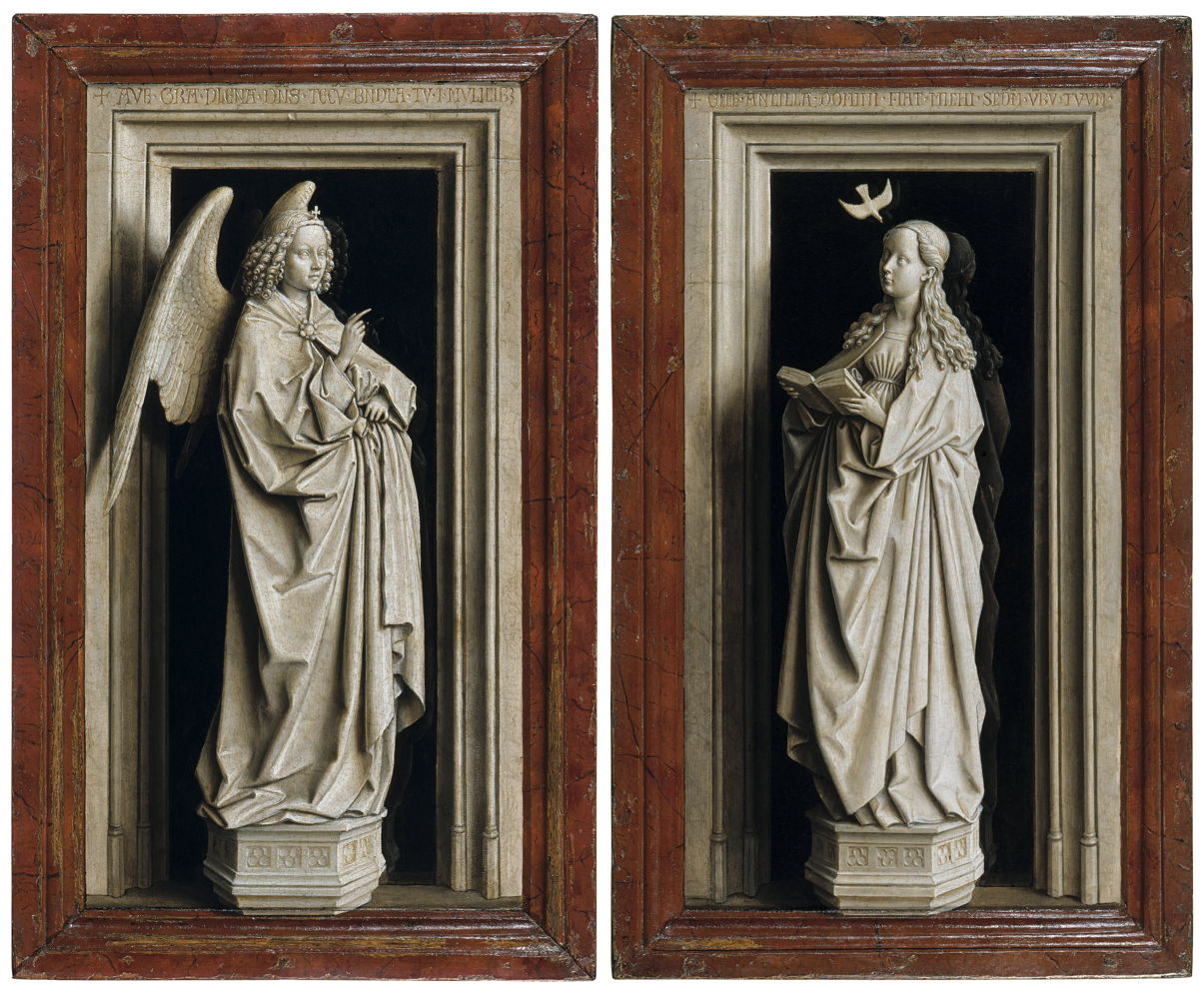
Jan van Eyck (c 1390–1441), The Annunciation Diptych (c 1433-35), oil on panel, dimensions not known, Museo Thyssen-Bornemisza, Madrid, Spain. Wikimedia Commons.
In the early Renaissance, before the stereotype could set in, there was greater innovation. For example, in about 1433-35 Jan van Eyck developed a monochrome grisaille into this brilliant trompe l’oeil, pretending to be a pair of sculpture figures in stone with wooden frames.
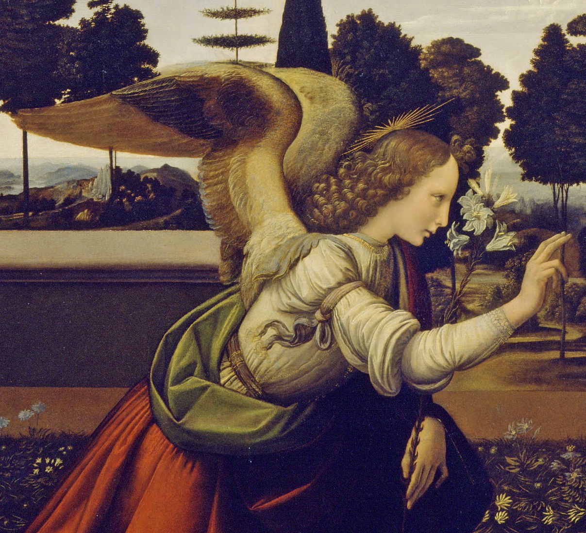
Leonardo da Vinci (1452–1519), Annunciation (c 1473-75), oil and tempera on poplar, 100 x 221.5 cm, Galleria degli Uffizi, Florence, Italy. Wikimedia Commons.
This Annunciation, painted in oil and tempera on a poplar panel, is generally agreed to be one of the earliest of Leonardo da Vinci’s own surviving paintings. When it was painted is in greater doubt, but a suggestion of around 1473-75 seems most appropriate. It shows his teacher Verrocchio’s influence, coupled with the less confident hand of a new master.
There are numerous pentimenti, particularly in the head of the Virgin. Its perspective projection is marked in scores in its ground. Nevertheless, Leonardo used his spontaneous and characteristic technique of finger-painting in some of its passages. Its composition and execution are conventional and conform to those seen in the output of Verrocchio’s workshop, complete with finicky detail throughout.
Leonardo da Vinci (1452–1519), Annunciation (detail) (c 1473-75), oil and tempera on poplar, 100 x 221.5 cm, Galleria degli Uffizi, Florence, Italy. Wikimedia Commons.
As is conventional, the Virgin Mary is sat reading her book, shown in detail down to lines of its text. The lectern is draped in a diaphanous fabric similar to the wraps seen in Verrocchio’s Madonnas.
Leonardo da Vinci (1452–1519), Annunciation (detail) (c 1473-75), oil and tempera on poplar, 100 x 221.5 cm, Galleria degli Uffizi, Florence, Italy. Wikimedia Commons.
The Archangel Gabriel is seen in profile, holding the usual white lily, and the details of his clothing, the flowers, and surrounds are all painted meticulously.
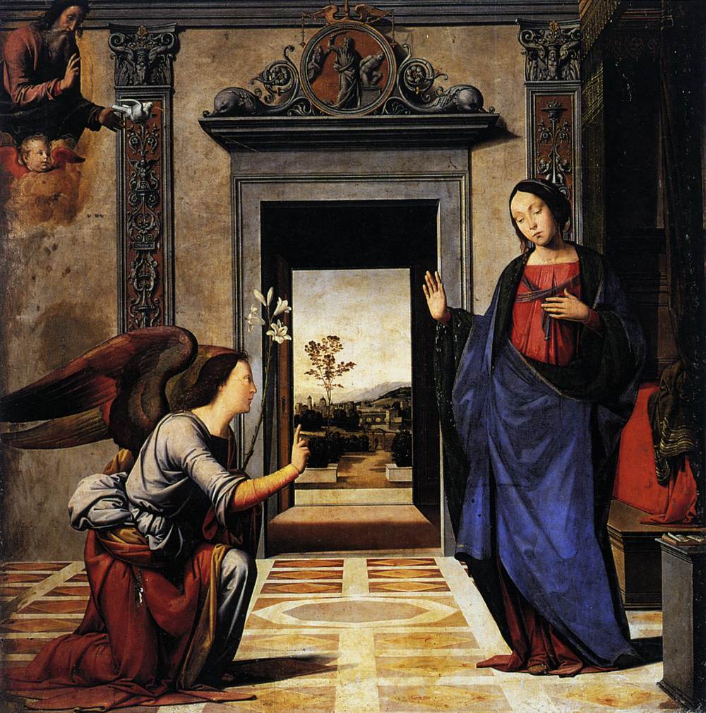
Fra Bartolomeo (1472–1517), The Annunciation (1497), oil on panel, 176 x 170 cm, Duomo di Santa Maria Assunta, Volterra, Italy. Wikimedia Commons.
The Annunciation (1497) is visibly one of Fra Bartolomeo’s earliest works, showing the Virgin Mary at the right being told by the angel Gabriel, at the left, that she would conceive Jesus Christ. Bartolomeo’s modelling of flesh is here unsophisticated, but the folds of garments are more advanced, as is his cameo landscape, suggesting influence from the Northern Renaissance. His perspective projection, shown in the floor patterning and the doorways, doesn’t quite resolve to a single vanishing point.
Gerard David (c 1450/1460–1523), The Annunciation (c 1510), oil on oak panel, 86.4 x 27.9 and 86.4 x 28.3 cm, Metropolitan Museum of Art, New Tork, NY. Wikimedia Commons.
In about 1510 Gerard David painted this diptych of The Annunciation in a style developed from the popular grisailles of the time. At the left is the Archangel Gabriel, with the Virgin Mary on the right. Instead of constraining himself to a true grisaille, David uses colours sparingly to enhance the effect.
Domenico di Pace Beccafumi (1486–1551), The Annunciation (1545-46), tempera on panel, 237 × 222 cm, Chiesa di San Martino in Foro, Sarteano, Italy. Wikimedia Commons.
About thirty-five years later, Beccafumi used the extreme contrast of chiaroscuro to heighten the effect of his painting, anticipating the vogue that was to come some fifty years later in the work of Caravaggio and his followers.
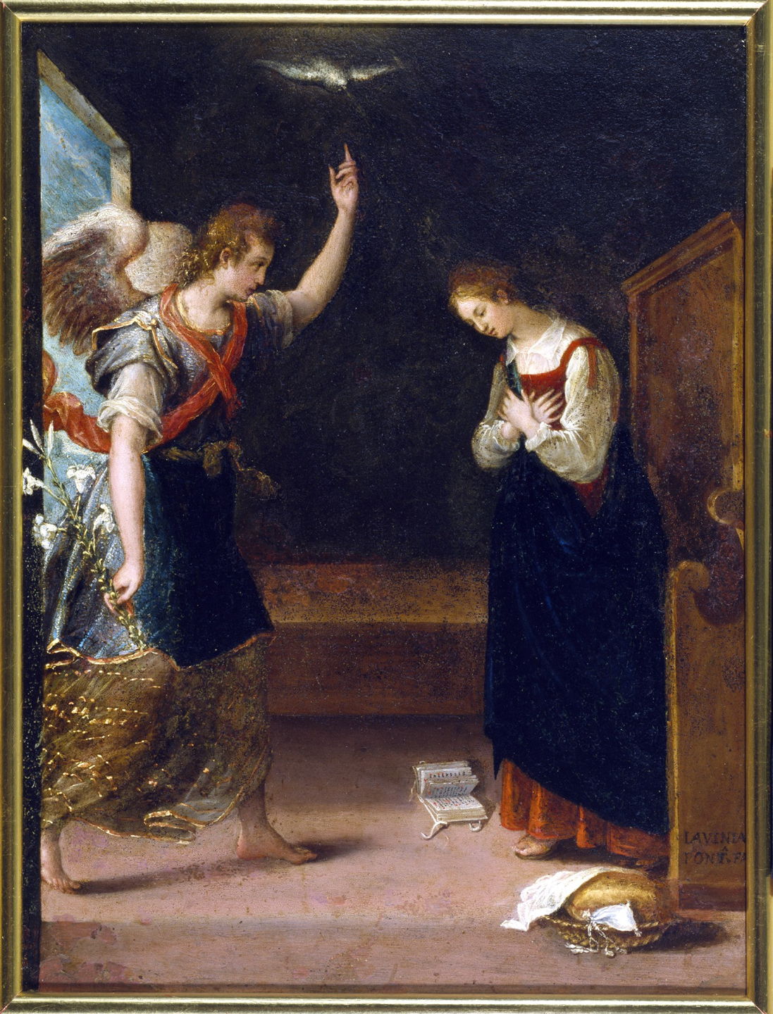
Lavinia Fontana (1552–1614), The Annunciation (c 1575), oil on copper, 36 x 27 cm, Walters Art Museum, Baltimore, MD. Courtesy of Walters Art Museum.
Several of Lavinia Fontana’s early paintings, including The Annunciation (c 1575), were made using oil on copper, an expensive and technically challenging support implying that they had already been commissioned by the more wealthy. This is a naturalistic depiction with the white dove symbolising the Holy Spirit, and traditional floral attributes.
Jacopo Tintoretto (c 1518-1594), The Annunciation (E&I 264) (c 1582), oil on canvas, 440 x 542 cm, Sala terrena, Scuola Grande di San Rocco, Venice, Italy. Wikimedia Commons.
Jacopo Tintoretto turned quite social-realist in this version from about 1582, with its unusually natural rendering of contemporary brickwork, a wicker chair, and a splendidly detailed carpenter’s yard at the left. This shows Christ’s origins as very real, tangible, and contemporary, a concept that didn’t reappear for over two centuries, as we’ll see tomorrow.
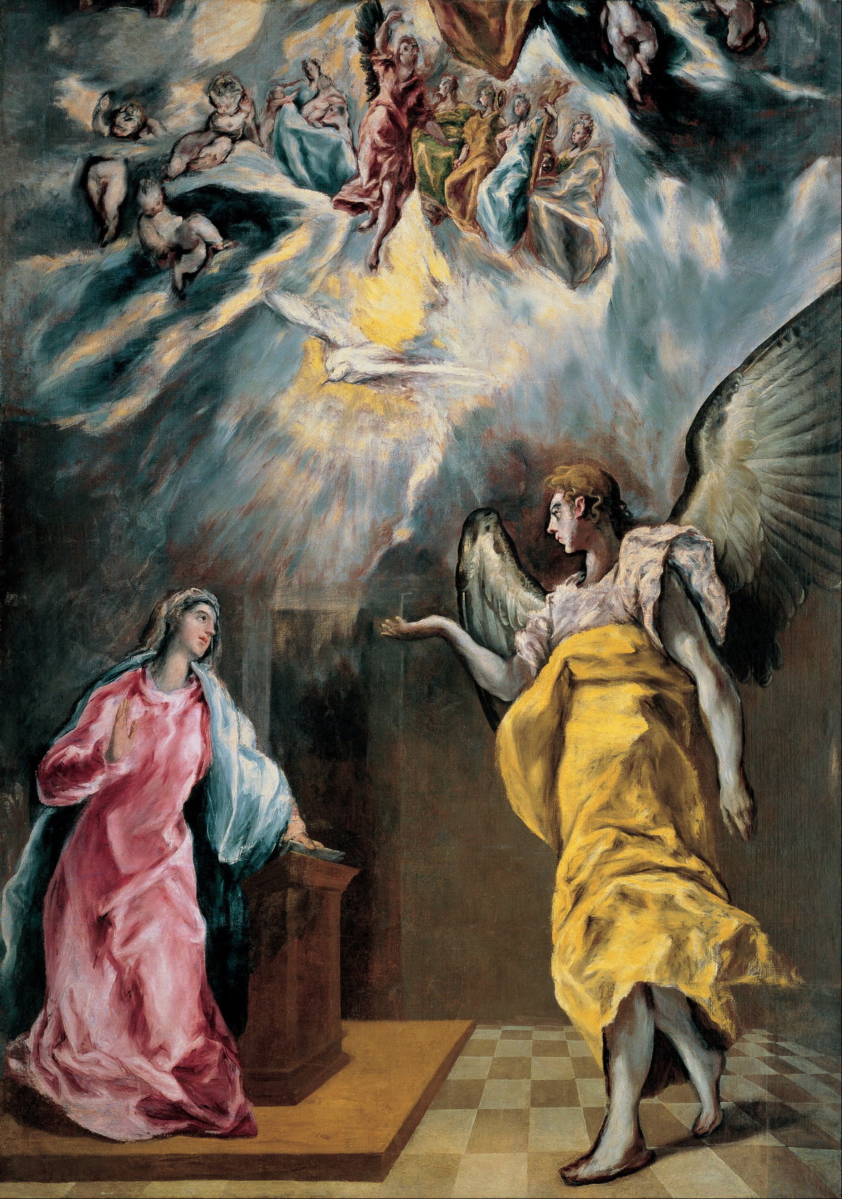
El Greco (Doménikos Theotokópoulos) (1541–1614), The Annunciation (1614), oil on canvas, 294 x 209 cm, Fundación Banco Santander, Madrid. Wikimedia Commons.
In 1614, El Greco used this unconventional composition, placing the figures in more expressive poses, with eloquent body language. The white dove is flying from a gaping light in the heavens, with a host of mothers and babies above. His brushwork is so painterly it could be mistaken for a much later work.
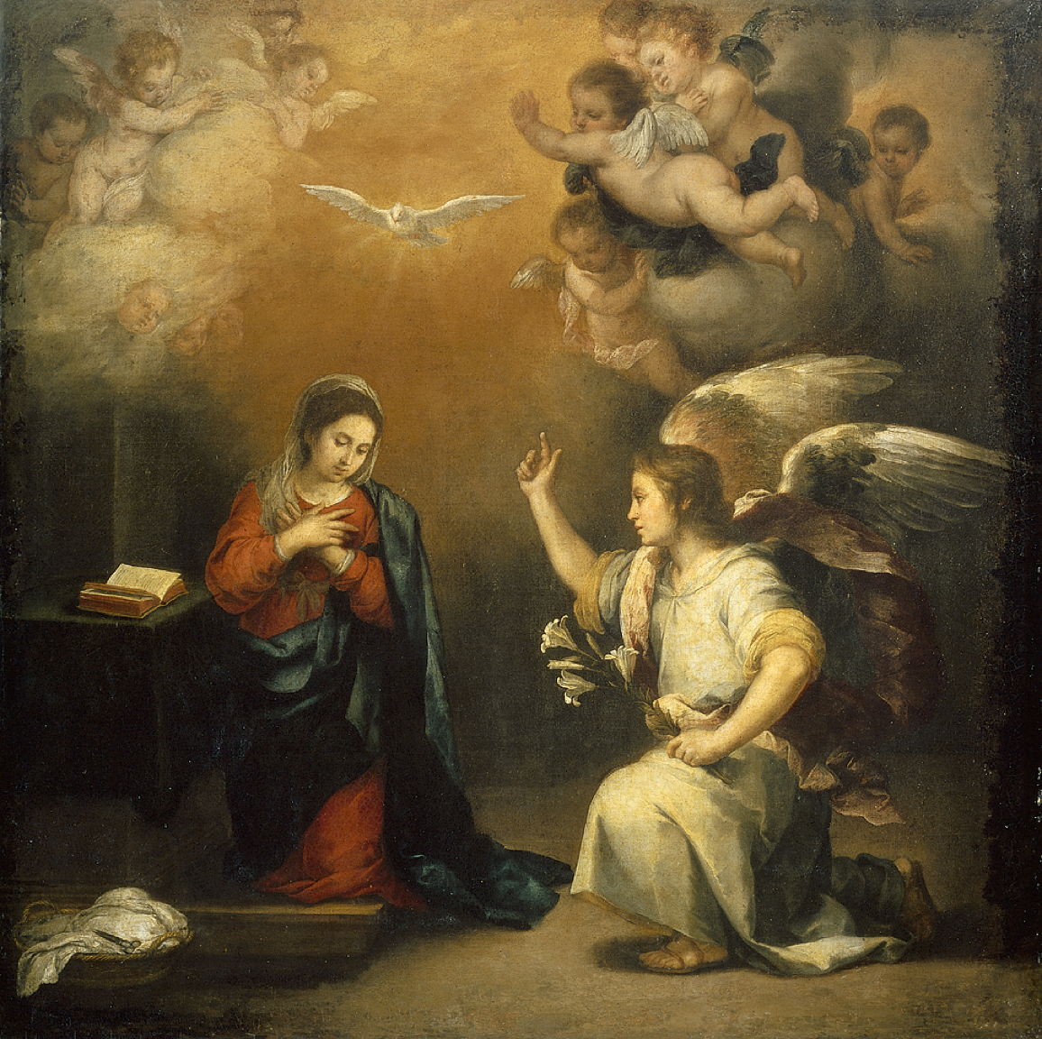
Bartolomé Esteban Murillo (1617–1682), The Annunciation (1660-80), oil on canvas, 98 x 100 cm, Rijksmuseum Amsterdam, Amsterdam, The Netherlands. Wikimedia Commons.
Murillo’s more conventional approach from 1660-80 is notable for the introduction of everyday props, such as the basket of linen under the table at the lower left corner, another herald of the depictions of the nineteenth century.
Storage information provided in macOS has a chequered history. While that provided in Disk Utility has remained a benchmark, a separate Storage feature introduced some years ago in About This Mac quickly became notorious for its fragility and inaccuracy, with many reporting huge discrepancies. Over the last couple of years, and with its transfer to System Settings > General > Storage, it has become more reliable and useful. This article explains where it has reached in macOS Tahoe 26.2.
Its view has three sections.
At the top, the Storage Bar shows a breakdown of space used on the boot disk into categories, total used, and total free space that now correlate better with figures shown in Disk Utility. The All Volumes button extends that to cover other disks, but as no detailed information is provided for them, you’re still better off checking in Disk Utility.
Recommendations
Below the Storage Bar comes a series of actions you could take to free up space. These operate across more than one category, but have limited usefulness:
Store in iCloud includes standard options such as putting your Desktop and Documents folders into iCloud Drive, and enabling iCloud Photo Library, which you’ve probably already decided on.
Optimise Storage isn’t the same as the Optimise Mac Storage option in iCloud Drive. What it does is remove the TV content that you’ve already watched from local storage.
Empty Trash Automatically simply deletes anything left in the Trash after a period of 30 days, an option also offered in the Finder’s Settings. Some love it, others manage by themselves.
Categories
The remainder of the view is devoted to individual categories, most of which are used to label segments of the Storage Bar. For most there’s an ⓘ Info button at the right, and in some cases that offers useful tools.
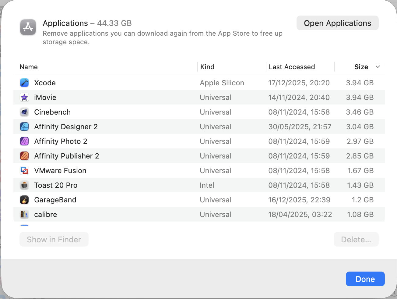
Applications can be listed by size or date of last access, making it easy to remove them. The total size given, and this list, excludes those apps bundled in the SSV, as they can’t be tampered with.
Books, Music, Music Creation and TV each let you delete local copies of content you have licensed, allowing you to download them later when you wish.
Developer can clean up some of the potentially redundant build and device support files accumulated by Xcode.
Documents offers lists of documents to show largest files, older downloads, unsupported 32-bit apps, and a file browser using column view sorting files by size. If you don’t want to use one of the third-party products that do this better, you may find this helpful, but it’s inferior to the likes of DaisyDisk and GrandPerspective.
Info offered for other categories includes:
iCloud Drive to enable Desktop and Documents in iCloud, also offered in numerous other places.
iOS files to remove unwanted device backups and firmware if you sync them with your Mac.
Mail adds nothing.
Messages is frustrating, as it lists large attachments, but when you try to preview them in the Finder, QuickLook refuses to oblige, so you can’t see what each is.
Photos can enable iCloud Photos, as offered elsewhere. Note that, as far as this category is concerned, the size given is that of the current System Photo Library, and excludes all other Photos Libraries and images in the Pictures folder.
Podcasts adds nothing.
Trash (or localised equivalents) lists items there for you to delete them, much as the Trash itself does.
Other Users & Shared covers Home folders of other users and any shared files.
macOS reveals how much space is being used by components supporting AI.
System Data is the one category that desperately needs further information, but doesn’t have a button. It’s discussed below.
Throughout these, Storage shows space actually taken on disk, rather than the nominal size. So a 100 GB VM stored as a sparse file might be shown as occupying only 62 GB, for example.
System Data
Storage appears to total all other categories up and account for the remainder of storage used in the category System Data. That doesn’t include the size of the System volume, or its snapshot, but can include temporary files like caches, snapshots, and anything else it can’t account for elsewhere.
In this case, System Data is by far the largest of all the categories, and accounts for half the space used on this SSD. This remains the greatest weakness in Storage settings, as the only way to discover and recover any of that space is to return to Disk Utility for its greater accuracy, its listing of snapshots, and of purgeable space. Even then, identifying what is using all that free space may end up as a process of elimination.
Let’s hope that Apple continues to improve Storage settings and provides more help to deal with System Data.
At the outbreak of war in 1914, the former Nabi painter and print-maker Félix Vallotton had turned to painting unusual landscapes showing transient atmospheric effects like fog, with the simplification of prints. He volunteered for the army, although he was rejected as he was almost fifty.
Félix Vallotton (1865–1925), The Sheaves (1915), oil on canvas, dimensions not known, Private collection. Wikimedia Commons.
Vallotton’s The Sheaves from 1915 is one of his moving and symbolic images of the Great War. It’s late summer, harvest time, and the ripe corn is being cut and stacked in sheaves. But where are those farmworkers, whose rakes rest against the sheaves, and whose lunch-basket sits on the ground ready to be eaten? Where is the wagon collecting the harvest, and why is the white gate in the distance closed?
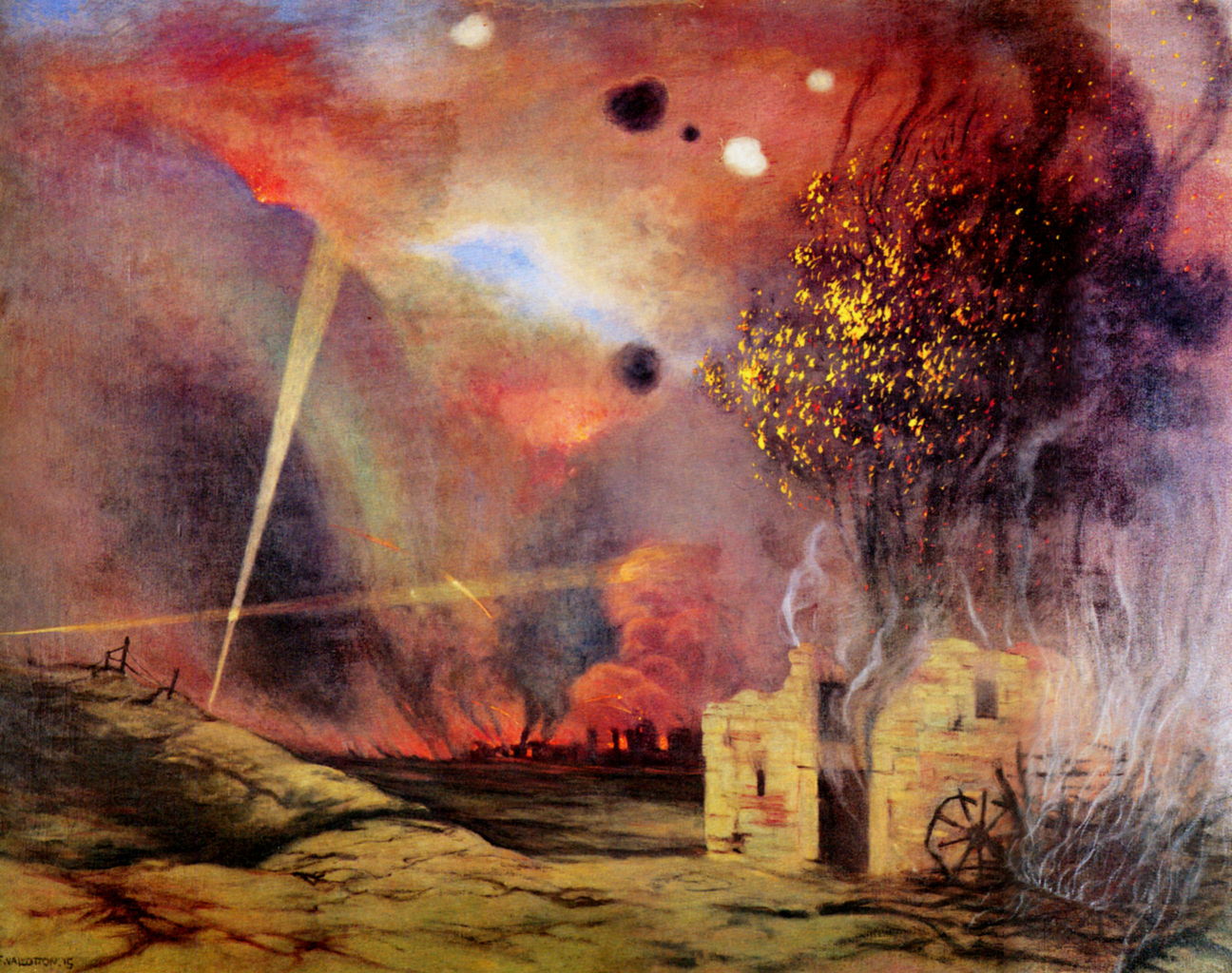
Félix Vallotton (1865–1925), Landscape of Ruins and Fires (1915), oil on canvas, 115.2 x 147 cm, Kunstmuseum Bern, Bern, Switzerland. Wikimedia Commons.
Then followed images of war itself. Landscape of Ruins and Fires from 1915 captures the utter destruction on the ground and surrealist displays in the sky. He returned to making woodcut prints, which he assembled into his last print series titled This is War.
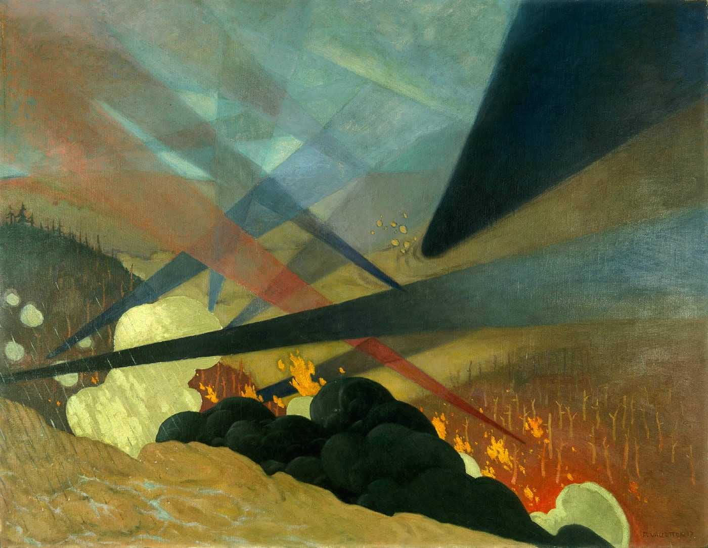
Félix Vallotton (1865–1925), Verdun (1917), oil on canvas, 114 x 146 cm, Musée de l’Armée, Hôtel des Invalides, Paris. Wikimedia Commons.
In 1917, he was commissioned as a War Artist to tour and paint the front line in Champagne, in the north-east of France. Verdun (1917) is one of the paintings he made as a result, where he shows the land burning under beams of coloured smoke, reversing their more usual appearance as beams of light. The Battle of Verdun, fought on the banks of the River Meuse, was the longest battle of the war, ending just before Christmas in 1916 with over 300,000 dead.
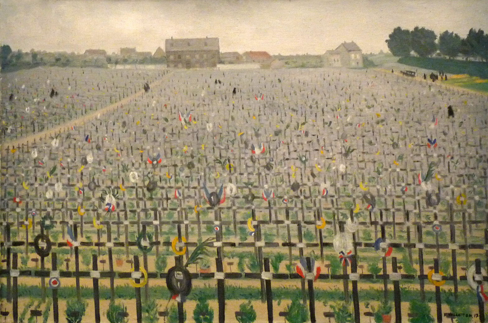
Félix Vallotton (1865–1925), Châlons War Cemetery (1917), oil on canvas, 54 x 80 cm, La contemporaine, Nanterre, France. Image by Ji-Elle, via Wikimedia Commons.
Perhaps Vallotton’s most moving painting of the First World War is his view of Châlons War Cemetery from 1917, with its countless rows of crosses receding into the town of Châlons-en-Champagne. There are a total of more than 4,500 French war graves from the First World War here, with other nationalities, and even more were added from the Second World War.
Félix Vallotton (1865–1925), Sunset at Grasse (1918), oil on canvas, 54 x 73 cm, Private collection. Wikimedia Commons.
Like Pierre Bonnard, Vallotton visited the town of Grasse, in the hills north of Cannes on the Mediterranean coast of France. In 1918, as one of a series of sunset views, he painted Sunset at Grasse with its saturated colours.
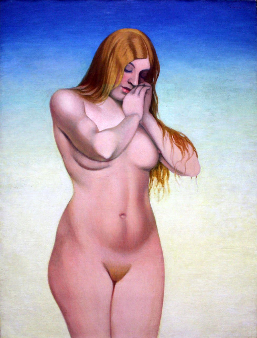
Félix Vallotton (1865–1925), Blonde Nude (1921), media and dimensions not known, Städelsches Kunstinstitut und Städtische Galerie, Frankfurt, Germany. Wikimedia Commons.
He continued to make some figurative paintings after the war. His Blonde Nude from 1921 develops the sleek, modern look from that of Le Bain turc in 1907.
Félix Vallotton (1865–1925), Chaste Suzanne (1922), oil on canvas, 54 x 73 cm, Musée cantonal des beaux-arts, Lausanne, Switzerland. Wikimedia Commons.
He still painted some narrative works too. When I first saw his Chaste Suzanne from 1922, I was puzzled as to what its story could be, but I think that this is a modern retelling of the Old Testament tale of Susanna and the Elders, where the two men are trying to blackmail Susanna into being unfaithful.
In the last few years of his life, like some other artists, he turned to landscapes. Unlike Ferdinand Hodler, he couldn’t paint these from his balcony, but seems to have gone back to his notebooks and sketches and painted composite views, similar to the ‘reminiscences’ of earlier landscape artists like Corot.
Félix Vallotton (1865–1925), The Old Olive Tree (1922), oil on canvas, 72 x 60 cm, Musée du Petit Palais, Geneva, Switzerland. Wikimedia Commons.
The Old Olive Tree from 1922 could be almost anywhere in southern Europe, although the stack of cut reeds resting against the tree adds a slightly surreal effect. In the distance, the terraced fields on the hillsides are brown and parched from the summer heat.
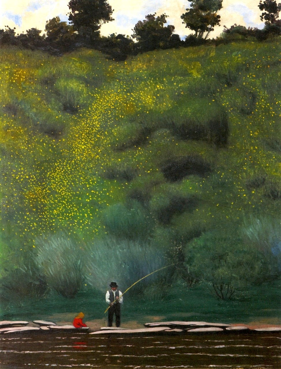
Félix Vallotton (1865–1925), Broom in Bloom, Avallon (1923), oil on canvas, 72.8 x 54 cm, Private collection. Wikimedia Commons.
Broom in Bloom, Avallon from 1923 shows an idyllic scene of fishing beside the river near the appropriately-named Avallon, which is south-east of Paris, towards Dijon and the Alps.
Félix Vallotton (1865–1925), Château Gaillard at Andelys (1924), oil on canvas, 82 x 65 cm, Musée cantonal des beaux-arts, Lausanne, Switzerland. Wikimedia Commons.
Vallotton painted this view of Château Gaillard at Les Andelys in 1924. The ruins of this mediaeval castle tower above this village in northern France. Les Andelys was popular with landscape painters during the nineteenth century, and was famous as Nicolas Poussin’s birthplace.
Félix Vallotton (1865–1925), The Dordogne at Carennac (1925), oil on canvas, 60 x 73 cm, Kunsthaus Zürich, Zürich, Switzerland. Wikimedia Commons.
The last of these wonderful print-inspired landscapes shows The Dordogne at Carennac, in the south-west of France, and dates from 1925.
By this time, he had completed over 1,700 paintings and some 200 prints. He then fell ill with cancer, and died that year, the day after his sixtieth birthday. His last novel, which he had started in 1907, was published posthumously.
I will conclude this short series with a summary after Christmas, to mark the centenary of his death.
It’s a simple question: which users can upgrade macOS? It was put to me by Cory, whose son had apparently upgraded their family Mac mini M4 to Tahoe from his standard user account. This article explains how that came about.
Upgrade or update?
Although the two words are sometimes used loosely, in strict senses updating takes macOS up in minor version or patch number, such as 26.0.1 to 26.1 or 26.2, while upgrading moves up to a newer major version, say from 15.7.2 to 26.2. Apple still makes this clear distinction too, although it has all become blurred.
Before it released macOS 12.3, upgrades were different from updates. For a Mac to be upgraded to a new major version, a full installer was downloaded and run, and that required an admin user to authenticate the installation. Updates were smaller and simpler, downloaded through Software Update, and could be installed by any user (apart from Guest).
For the last three years, with the upgrades to Ventura, Sonoma, Sequoia and now Tahoe, whenever possible upgrades have been performed using the update method instead of a full installer. It’s significantly faster, with less to download, decompress and install. Although Apple still claims that “before installation begins, you’re asked to enter your administrator password”, that’s no longer correct, even on Apple silicon Macs.
Who can update macOS?
The requirements for a user to be able to update macOS are:
a standard or admin user account on that Mac, and
ownership of the boot volume group to be updated.
The first user, or primary admin user, on that Mac is granted a secure token to enable them to take ownership of the boot volume group on that Mac’s internal SSD. Rights of that ownership include
being able to change startup security policy for that boot volume group, using Startup Security Utility in Recovery mode;
authorising installation of macOS updates and upgrades;
being able to initiate Erase All Content and Settings (EACAS);
granting secure tokens and ownership to other users.
When that primary admin user creates another user account, a secure token and ownership is handed over to that account, even when it’s only a standard account. That enables subsequent users to automatically unlock FileVault at login, and to authorise the installation of macOS updates. As upgrades now work the same as updates, that means that standard users whose passwords can unlock FileVault (if enabled) can now authorise the installation of macOS upgrades as well as updates.
What do others say?
Search for answers to the question, and you’ll mostly see outdated accounts from before macOS 12.3, and those clearly influenced Google AI, which wrote:
“Any user with a Secure Token and volume ownership can install minor macOS updates (like 14.1 to 14.2), but major macOS upgrades (like Sonoma to Sequoia) typically still require an Administrator password, unless managed by an organization with specific Mobile Device Management (MDM) policies that grant permissions to standard users. Essentially, standard users can update, but major upgrades need admin power, though MDM can override this for managed devices.”
(For interest, Grok didn’t even understand the question, and simply listed models of Mac that can be upgraded to Tahoe.)
That has been wrong for over three years now, but that error is still widely propagated.
What can you do?
If you want to give another user access to your Mac as a standard user, but don’t want them to update and/or upgrade macOS, you will need to explain this to them, and caution them not to succumb to Apple’s aggressive schemes to trick users to upgrade.
In the first of these two articles looking at bread in visual art, I considered it as a symbol of life, predominantly following the Christian tradition set by the Last Supper. Here I consider bread in its role as food, the staple of most Europeans.
Jean-François Raffaëlli (1850-1924), Man with Two Loaves of Bread (1879), further details not known. Wikimedia Commons.
Man with Two Loaves of Bread (1879) is one of Jean-François Raffaëlli’s social realist paintings. This man’s bowed head and furtive look make you wonder just how he had acquired those loaves.
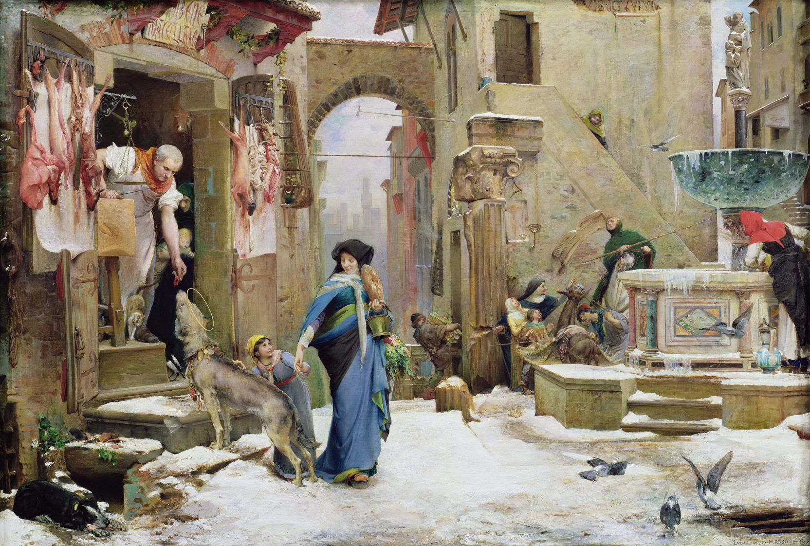
Luc-Olivier Merson (1846–1920), The Wolf of Agubbio (1877), oil on canvas, 88 x 133 cm, Palais des Beaux-Arts de Lille, Lille, France. Wikimedia Commons.
Luc-Olivier Merson’s wonderful painting of the Franciscan legend of The Wolf of Agubbio from 1877 is set in the town’s central piazza on a bitter winter’s day. The large wolf of the legend has a prominent halo and stands at the door of the butcher’s shop, from where the butcher is handing it a piece of meat. A young girl smiles open-mouthed as she strokes the wolf’s back. Her mother holds her other hand, as she walks back clutching a loaf of bread and other provisions (detail below).
Luc-Olivier Merson (1846–1920), The Wolf of Agubbio (detail) (1877), oil on canvas, 88 x 133 cm, Palais des Beaux-Arts de Lille, Lille, France. Image by Chatsam, via Wikimedia Commons.Johannes Vermeer (1632–1675), The Milkmaid (c 1658-59), oil on canvas, 45.5 x 41 cm, The Rijksmuseum Amsterdam, Amsterdam, The Netherlands. Wikimedia Commons.
Vermeer’s Milkmaid, probably from about 1658-59, is less about milk than the bread on the tabletop. A wicker basket of bread is nearest the viewer, broken and smaller pieces of different types of bread behind and towards the woman, in the centre. These are shown in the detail below, where Vermeer’s controlled use of blurring is visible.
Johannes Vermeer (1632–1675), The Milkmaid (detail) (c 1658-59), oil on canvas, 45.5 x 41 cm, The Rijksmuseum Amsterdam, Amsterdam, The Netherlands. Wikimedia Commons.
Perhaps because it was so commonplace in many households and bakers, there are relatively few paintings showing the making and baking of bread.
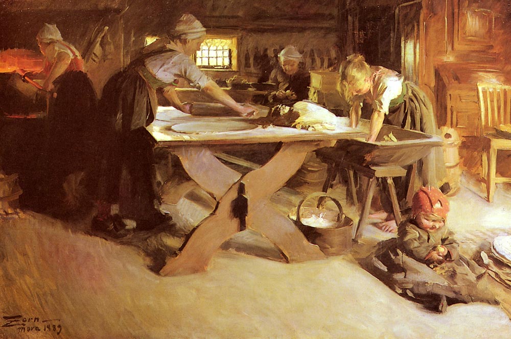
Anders Zorn (1860–1920), Baking Bread (1889), oil on canvas, dimensions not known, Private collection. WikiArt.
In Baking Bread, painted in Mora, the artist’s home town in Sweden in 1889, Anders Zorn captures each step in the process in documentary fashion, from kneading the dough, through rolling and preparing it, to its baking. There’s even an infant in the foreground who looks ready to be its consumer.
Helen Allingham (1848-1926), Baking Bread (date not known), watercolour, further details not known. The Athenaeum.
Helen Allingham’s undated Baking Bread shows a traditional farmhouse baking oven being used to bake the bread for an extended family, or possibly a small village shop. These ovens can still be found in many remaining period dwellings, but are now seldom used.
Christian Krohg (1852–1925), Woman Cutting Bread (1879), oil on canvas, 80 x 60 cm, Bergen kunstmuseum, Bergen, Norway. Wikimedia Commons.
Christian Krohg’s early painting of Ane Gaihede as a Woman Cutting Bread (1879) marked the start of his social realism. Krohg documents her in almost ethnographic detachment. She is aligned in profile, against an almost bare wall, perfectly framed at three-quarter length.
Finally, bread is occasionally featured in still life paintings.
Anne Vallayer-Coster (1744–1818), A Still Life of Mackerel, Glassware, a Loaf of Bread and Lemons on a Table with a White Cloth (1787), further details not known. Wikimedia Commons.
Anne Vallayer-Coster painted A Still Life of Mackerel, Glassware, a Loaf of Bread and Lemons on a Table with a White Cloth in 1787, when she was at her artistic zenith.
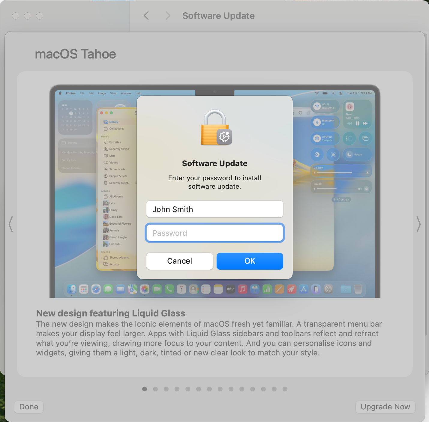
One of the primary aims of most malware is to trick you into giving it your password. Armed with that, there’s little to stop it gathering up your secrets and sending them off to your attacker’s servers. One of your key defences against that is to know when a password request is genuine, and when it’s bogus. By far the best way to authenticate now is using Touch ID, but many Macs don’t support it, either because they can’t, or because their keyboard doesn’t, and there are still occasions when a genuine request may not offer it. This article looks at the anatomy of a range of genuine password requests. Note that these dialogs aren’t generated by the app, but come from the macOS security system, hence their consistency.
Traditional, no Touch ID
This authentication dialog is very important: although malware might try to forge it, it contains distinctive features you should always look for:
The icon consists of a locked padlock, on which is superimposed a miniature icon representing the app or component that has asked to access the keychain.
The bold text names the app or component that has called for keychain access, and states which item it’s asking to access: here, a named secure note.
The smaller lettering specifies that it’s asking for the keychain password, that is the password used to unlock the named keychain, not that for your Apple Account or any other password.
If you’re in any doubt about its authenticity, click on the Deny button and the request will be denied.
If you’re in any doubt about its authenticity, open Keychain Access, lock the keychain there, and repeat the action while watching the keychain to ensure that it’s unlocked and handled correctly.
Note this doesn’t provide or ask for your user name, only the password for that keychain.
Vertical, no Touch ID
This newer vertical format should contain the following:
The icon consists of a locked padlock, on which is superimposed a miniature icon representing the app or component that is asking for your password.
Bold text names the app making the request.
Below that is a general indication of the purpose of the request.
Below that is the instruction to Enter your password to allow this.
There are two text boxes, to contain your user name (already completed) and password.
There are only two buttons, one of which may be OK or something more specific, and the other is Cancel.
If you’re in any doubt as to its authenticity, click on the Cancel button to deny the request, and consult the app’s documentation.
Here’s a similar version from Sequoia, seen in Dark Mode, with the same key features.
Touch ID
If your Mac supports Touch ID (all Intel Macs with T2 chips, and all Apple silicon Macs), and currently has a keyboard connected to it with support for Touch ID (Intel laptops and Apple silicon Macs only), macOS should offer you the biometric version of that authentication dialog.
This should contain the following:
The icon consists of a Touch ID fingerprint, on which is superimposed a miniature icon representing the app or component that is asking for your password.
Bold text names the app making the request.
Below that is a general indication of the purpose of the request.
Below that is the instruction to Touch ID or enter your password to allow this.
There are only two buttons, the upper being Use Password…, and the lower is Cancel.
If you’re in any doubt as to its authenticity, click on the Cancel button to deny the request, and consult the app’s documentation.
This dialog has distinctive behaviour that’s difficult to forge. When you place your fingertip on the Touch ID button on the keyboard, it will either authenticate successfully, so dismissing the dialog, or the dialog shakes to indicate you should try placing your fingertip on the button again.
Here’s a more recent version from Tahoe, with the icon and text left-justified.
You will also see the icon with its fingerprint whorls filled in colour.
If Touch ID authentication fails, or you click on the button to Use Password…, the dialog expands to resemble the non-biometric version above, with the following two important differences:
The icon still consists of a Touch ID fingerprint, with a superimposed miniature icon representing the app or component.
The instruction remains to Touch ID or enter your password to allow this.
Terminal
Authenticating in Terminal, typically when using sudo, has less scope for distinctive detail, and might appear simpler to forge. However, macOS has a couple of tricks up its sleeve that are difficult to fake.
This contains the following:
The prompt consists of the single word ending with a colon, Password: Other words, such as System password, are fakes.
Immediately after the colon is a distinctive icon of a vertical white key on a grey rectangle. The closest you’ll see in standard Unicode is the Squared Key character ⚿ which is obviously different.
As you type in your password, not only are the characters not shown, but the same key icon remains where it is, and there’s no indication on screen that you’re typing anything in until you press Return. Fakes usually display characters as you type them in.
Again, if you’re in any doubt, simply press Return and exit without giving any characters of your password away.
Finally, no matter how rushed you might be, or sick to death of repeated authentication requests, check every one carefully before typing anything in, as if your Mac’s security depended on it. Because it does.
Towards the end of each year, I take a look back at some of the paintings that were completed a century ago. In histories of painting, that was a time of late Cubism, Surrealism, Expressionism and abstraction, but most of those works remain protected by copyright. In this and the next two articles you will see a broader range of styles.
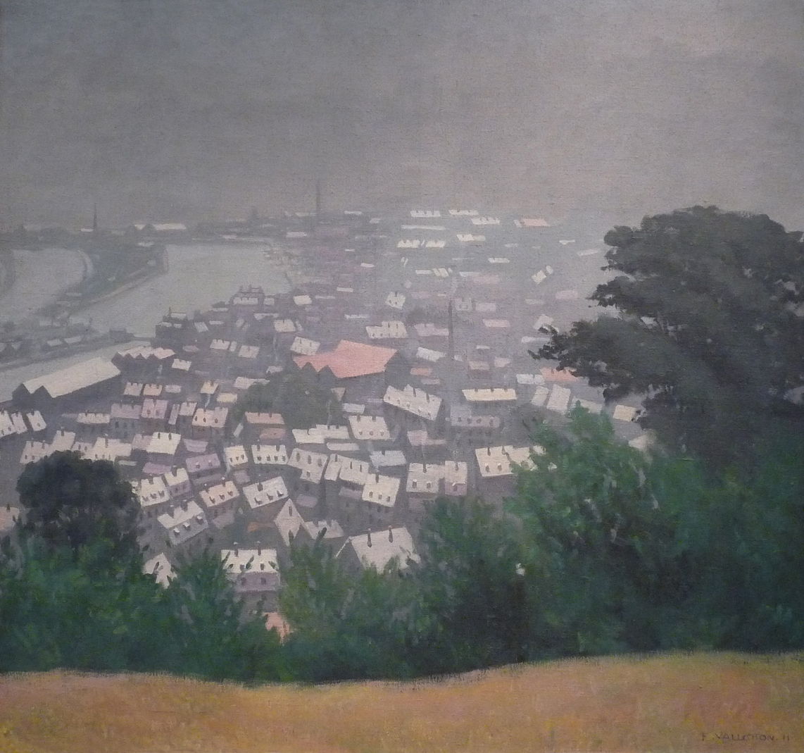
Laurits Andersen Ring (1854–1933), Ole Ring looks over Roskilde (1925), oil on canvas, 36.5 x 28 cm, Ordrupgaard, Jægersborg Dyrehave, Denmark. Wikimedia Commons.
When his son was twenty-three, the Danish painter LA Ring painted him in Ole Ring looks over Roskilde. This is reminiscent of Ring’s Young Girl Looking out of a Roof Window that he had painted in Copenhagen back in 1885, forty years earlier at the start of his career. The church shown here is, I believe, Roskilde Cathedral.
Félix Vallotton (1865–1925), The Dordogne at Carennac (1925), oil on canvas, 60 x 73 cm, Kunsthaus Zürich, Zürich, Switzerland. Wikimedia Commons.
In 1925, Félix Vallotton painted the last of his late landscapes, showing The Dordogne at Carennac. The town of Carennac is on the banks of the River Dordogne in the south-west of France.
From 1924 until 1930, Paul Signac spent most summers in Brittany, where he sketched and painted the island of Groix.
Paul Signac (1863-1935), Lighthouse at Groix (Cachin 568) (1925), oil on canvas, 74 x 92.4 cm, Metropolitan Museum of Art, New York, NY. Wikimedia Commons.
From those, he painted Lighthouse at Groix in the studio. This shows a tuna boat returning to port in the evening, by which time the rest of the fleet are drying their sails in harbour. This wasn’t exhibited until 1930. The detail below shows his evolving facture, which remained steadfastly pointillist in his oil paintings.
Paul Signac (1863-1935), Lighthouse at Groix (Cachin 568) (detail) (1925), oil on canvas, 74 x 92.4 cm, Metropolitan Museum of Art, New York, NY. Wikimedia Commons.Paul Signac (1863-1935), Le Pont des Arts (Paris) (Cachin 569) (1925), oil on canvas, 89 x 115 cm, Private collection. Wikimedia Commons.
From his Paris apartment, Signac sketched many views of the River Seine and its bridges in watercolour. From those came this painting of Le Pont des Arts (Paris), with its reference to his much earlier views of industrial sites along the river’s banks.
Paul Signac (1863-1935), Lézardrieux (1925), watercolour over Conté crayon, dimensions not known, Honolulu Museum of Art, Honolulu, HI. Wikimedia Commons.
He also combined Conté crayon (a proprietary type of hard pastel) with watercolour for this view of Lézardrieux. This is a village at the far western end of the French Channel coast, and a popular port with yachtsmen. He appears to have sharpened the Conté crayon to use it to sketch the outlines before applying watercolour wash, in a manner not unlike the late watercolours of Paul Cézanne.
Paul Signac (1863-1935), L’île-aux-Moines (1925), further details not known. Wikimedia Commons.
That year, he travelled south from there to the northern end of the Bay of Biscay, where he painted this view of L’île-aux-Moines, one of two islands off that section of the coast of Brittany.
While Signac was painting in the north-west, Pierre Bonnard was active in the far south.
Pierre Bonnard (1867-1947), View of Cannes (c 1925), oil on canvas, 28 x 55 cm, Private collection. The Athenaeum.
Most of Bonnard’s finest landscapes from this period, like this View of Cannes, were painted on or near the Mediterranean coast, in the special light of le Midi.
Pierre Bonnard (1867-1947), Boats at Antibes (1925), oil on canvas, 36.2 x 44.1 cm, Private collection. The Athenaeum.
Some local harbours there had become very popular during the summer, as he shows in Boats at Antibes.
The American artist Marsden Hartley returned to Europe in 1921, then based himself in Aix-en-Provence, Paul Cézanne’s home town, between about 1925-28.
Marsden Hartley (1877–1943), Landscape (1925), oil on panel, 36.8 x 46.4 cm, Herbert F. Johnson Museum of Art, Ithaca, NY. Wikimedia Commons.
Many of his landscapes from those years were strongly influenced by Cézanne’s later paintings, such as his Landscape. This shows extensive use of Cézanne’s constructive stroke, patches of parallel brushstrokes that are relatively independent of an object’s form.
Lesser Ury (1861–1931), Nollendorfplatz Station at Night (1925), media and dimensions not known, Märkisches Museum, Berlin, Germany. Image by anagoria, via Wikimedia Commons.
In Germany, Lesser Ury was continuing his successful urban nocturnes with his masterly oil sketch of Nollendorfplatz Station at Night. This busy railway station is to the south of the Tiergarten, in one of Berlin’s shopping districts.
Extended attributes (xattr) contain a wide range of metadata, some of which are intended to persist with the file they’re attached to, others to be more transient. Depending on the type of file operation performed, macOS has an elaborate mechanism for determining which are preserved, and which are not. This article tries to explain how this works in macOS Tahoe 26.0.
Xattr flags
When first introduced in Mac OS X, no provision was made for xattrs to have type-specific preservation, and that was added later using flags suffixed to the xattr’s name. For example, the com.apple.lastuseddate xattr found commonly on edited files is shown with a full name of com.apple.lastuseddate#PS to assign the two flags P and S to it, and the most recent xattr com.apple.fileprovider.pinned, used to mark files in iCloud Drive that have been pinned, has the two flags P and X assigned to it for a the full name of com.apple.fileprovider.pinned#PX.
This is a kludge, because you normally have to refer to the xattr name including its flags, although the flags aren’t really part of its name. This can catch the unwary.
It’s further complicated by a set of system tables for some standard xattr types that don’t have flags suffixed, but are treated as if they do. One notable example of those is the quarantine xattr com.apple.quarantine, which is handled by macOS as if it has the PCS flags attached, although those are never used when referring to it by name.
There are also lower case flags that can be used to override those set in system tables, although those appear to be used exceedingly rarely, and I don’t recall ever coming across them. In theory, if you were using a new type based on the standard com.apple.metadata: family, com.apple.metadata:kMDItemNew, you could alter its behaviour to some similar types with the flags psB, as in com.apple.metadata:kMDItemNew#psB. I have no idea whether that would be respected in practice. For the rest of this article, I will ignore the existence of those lower case flags.
Intents
File operations involving decisions about the preservation of xattrs are simplified into the following intents:
copy – simply copying a file from a source to a destination and preserving its data, such as using cp, is labelled XATTR_OPERATION_INTENT_COPY
save – saving a file when probably changing its content, including performing a ‘safe save’; this may over-write or replace the source with the saved file. Some xattrs shouldn’t be preserved in this process of XATTR_OPERATION_INTENT_SAVE
share – sharing or exporting this file, perhaps as an attachment to email, or placing the file in a public folder. Some sensitive metadata shouldn’t be preserved in XATTR_OPERATION_INTENT_SHARE
sync – syncing the file to a service such as iCloud Drive, in XATTR_OPERATION_INTENT_SYNC
backup – backing the file up, perhaps using Time Machine, in XATTR_OPERATION_INTENT_BACKUP.
Flags
As of macOS 15.0 (including 26.0), the following flags are supported:
C: XATTR_FLAG_CONTENT_DEPENDENT ties the flag with the file contents, so the xattr has to be recreated when the file data changes. This may be appropriate for checksums and hashes, text encoding, and position information. The xattr is then preserved for copy and share, but not in a safe save.
P: XATTR_FLAG_NO_EXPORT doesn’t export or share the xattr, but preserves it during copying.
N: XATTR_FLAG_NEVER_PRESERVE ensures the xattr is never preserved, even when copying the file.
S: XATTR_FLAG_SYNCABLE ensures the xattr is preserved during syncing with services such as iCloud Drive. Default behaviour is for xattrs to be stripped during syncing, to minimise the amount of data to be transferred, but this flag overrides that.
B: XATTR_FLAG_ONLY_BACKUP keeps the xattr only in backups, including Time Machine, where there’s no desire to minimise what’s backed up.
X: XATTR_FLAG_ONLY_SAVING keeps the xattr only when saving and in backups, including Time Machine (macOS 15.0 and later only).
There’s another system limit that must be adhered to: total length of the xattr name including any # and flags cannot exceed a maximum of 127 UTF-8 characters.
System tables
These are hard-coded in source, where * represents a ‘wild card’:
com.apple.quarantine – PCS preserved in copy, sync, backup
com.apple.metadata:kMDItemCollaborationIdentifier – B backup
com.apple.metadata:kMDItemIsShared – B backup
com.apple.metadata:kMDItemSharedItemCurrentUserRole – B backup
com.apple.metadata:kMDItemOwnerName – B backup
com.apple.metadata:kMDItemFavoriteRank – B backup
com.apple.metadata:* (except those above) – PS copy, save, sync, backup
com.apple.security.* – S or N depending on sandboxing, see below
com.apple.ResourceFork – PCS copy, sync, backup
com.apple.FinderInfo – PCS copy, sync, backup
com.apple.root.installed – PC copy, backup.
System defaults for com.apple.security.* depend on whether the app performing the file operation is running in an app sandbox. Non-sandboxed apps apply S to preserve the xattr for copy, save, share, sync, backup; for sandboxed apps N is applied so the xattr is never preserved, even when copying the file.
Flags and intents
We can now revisit the list of intents, and establish the effects of xattr flags on each, as:
XATTR_OPERATION_INTENT_COPY preserves xattrs that don’t have flag N or B or X
XATTR_OPERATION_INTENT_SAVE preserves xattrs that don’t have flag C or N or B
XATTR_OPERATION_INTENT_SHARE preserves xattrs that don’t have flag P or N or B or X
XATTR_OPERATION_INTENT_SYNC preserves xattrs if they have flag S, or have neither N nor B
XATTR_OPERATION_INTENT_BACKUP preserves xattrs that don’t have flag N.
Finally, Apple provides separate information on how xattrs are synced by FileProvider, for iCloud Drive and third-party cloud services using that API. This confirms that the S flag should sync a xattr, but is vague on other flags, simply stating “some older attributes are also synced”. However, a cap is applied on the maximum size of xattrs that are syncable, at “about 32KiB total for each item”. If the xattrs exceed that limit “the system automatically makes some of the attributes nonsyncable.” More puzzlingly, it states “the resource fork is content and isn’t included in the extended attributes dictionary.”
Conclusions
Controls over the preservation of xattrs are appended as tags to their name, following a hash #. In most circumstances, they should be treated as part of that xattr’s name, and are required for commands and actions on that xattr, for example when using the xattr command. They should also be left intact and not removed, unless you want to change the behaviour of that xattr in file operations.
Most xattrs commonly used by macOS don’t explicitly use tags, but are governed by a hard-coded system table that can’t be changed.
When using standard commands such as cp, macOS will automatically apply these rules when deciding whether to preserve xattrs. However, using a command for a different intent, such as cp for backing up, won’t normally invoke the behaviour you might want.
Code using standard macOS file operations should follow the behaviour expected for its intent, and shouldn’t require any special handling of xattrs. Lower-level operations are likely to differ, though, and may require implementation of equivalent behaviours.
Those implementing their own xattr types should incorporate flags explicitly to ensure they’re preserved as intended.
In cases of uncertainty, for example when working with files stored in iCloud Drive, you’ll need to step carefully through the rules above.
Sources
xattr_flags.h, xattr_flags.c, xattr_properties.h in copyfile source, e.g. at Apple’s OSS Distributions Github
man xattr_name_with_flags(3), included in copyfile source FileProvider (Apple).
Apple has just released an update to XProtect, bringing it to version 5325. As usual, it doesn’t release information about what security issues this update might add or change.
This version adds five new Yara rules, four for the Soma/Amos family – MACOS.SOMA.DEENA, MACOS.SOMA.DEPEA, MACOS.SOMA.DETRA, and MACOS.SOMA.DELEA – and MACOS.ODYSSEY.DEENA for the Odyssey family.
You can check whether this update has been installed by opening System Information via About This Mac, and selecting the Installations item under Software.
A full listing of security data file versions is given by SilentKnight and SystHist for El Capitan to Tahoe available from their product page. If your Mac hasn’t yet installed this update, you can force it using SilentKnight or at the command line.
If you want to install this as a named update in SilentKnight, its label is XProtectPlistConfigData_10_15-5325
Sequoia and Tahoe systems only
This update has not yet been released for Sequoia and Tahoe via iCloud, but should be shortly. If you want to check it manually, use the Terminal command sudo xprotect check
then enter your admin password. If that returns version 5325 but your Mac still reports an older version is installed, you should be able to force the update using sudo xprotect update
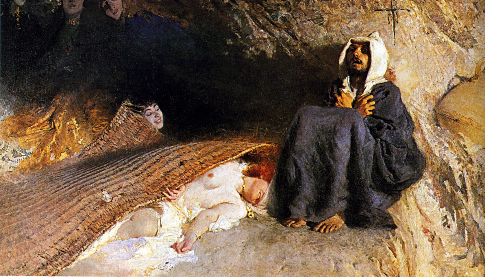
Paulus Bor (1601-1669) was born in the city of Amersfoort, to the north-east of Utrecht, and seems to have started his training locally before going to Rome, where he was one of the founders of a ‘secret’ society of Netherlandish expatriates, the Bentvueghels (‘birds of a feather’). He returned to Amersfoort to perform some decorative painting, then pursued a successful career there until his death in 1669. Apart from a Caravaggist tendency during his early career, he might seem a run-of-the-mill painter of the Golden Age.
What distinguishes Bor are his little-known portraits of women in trouble, images that dig deep into the psyche, long before the Age of Enlightenment.
Paulus Bor (circa 1601–1669), Ariadne (1630-35), oil on canvas, 149 x 106 cm, Muzeum Narodowe w Poznaniu, Poznań, Poland. Wikimedia Commons.
The first of these is Ariadne, painted in the period 1630-35, which is reminiscent of Caravaggio, and a little mysterious. When Theseus came to Crete to kill the Minotaur, Ariadne helped him by giving him a ball of golden thread that he used to retrace his route out of the labyrinth after he had killed the Minotaur (her half-brother). Ariadne fell in love with Theseus, and the couple eloped to Naxos, where he abandoned her.
Bor’s portrait can only show Ariadne on Naxos, immediately after she has been abandoned, still clutching the thread by which she thought she had tethered Theseus, now hanging at a loose end. On the wall above her are sketches she has made of her lover. She looks deeply lost in thought and gloom. This may refer to Ovid’s imaginary letter from her to Theseus in his Heroides.
Paulus Bor (c 1601–1669), The Magdalen (c 1635), oil on wood panel, 65.7 x 60.8 cm, Walker Art Gallery, Liverpool, England. Wikimedia Commons.
Then, in about 1635, Bor painted The Magdalen, clutching her bottle of myrrh and looking straight at the viewer. She too is troubled, and has clearly been crying.
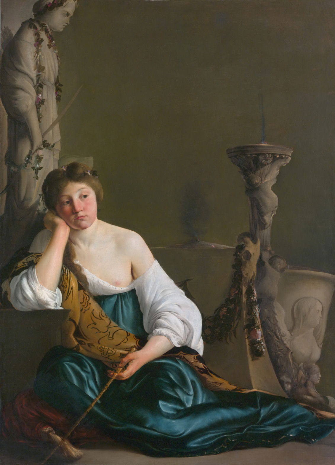
Paulus Bor (c 1601–1669), Allegorical Figure (Allegory of Logic) (c 1635), oil on canvas, 81.7 x 70 cm, Musée des Beaux-Arts de Rouen, Rouen, France. Image by Caroline Léna Becker, via Wikimedia Commons.
At about the same time, he painted this Allegorical Figure, also known as an Allegory of Logic. Coiled around her right wrist is a snake, but she too looks straight at you. The reptile appears venomous, and could easily be a European adder (or viper), or even an asp of the type Cleopatra used to kill herself.
Bor’s last two portraits of women in trouble have clearer narrative bases.
Paulus Bor (c 1601–1669), The Disillusioned Medea (The Enchantress) (c 1640), oil on canvas, 155.6 x 112.4 cm, The Metropolitan Museum of Art, New York, NY. Wikimedia Commons.
The Disillusioned Medea (The Enchantress) from about 1640 appears unique among the images of the enchantress who used her magic to support Jason in his quest for the Golden Fleece. She fell in love with Jason, married him on his voyage home, and bore him two children. Ten years later, Jason divorced her for the King of Corinth’s daughter Glauce.
This was too much for Medea, who sent Glauce a poisoned wedding dress that killed her and her father horribly. She then killed her two children, and fled to Athens, where she had a child by King Aegeus. Ovid includes an imaginary letter from her to Jason in his Heroides.
Medea sits, her face flushed, resting her head on the heel of her right hand. In her left, she holds a wand made from bamboo or rattan. The wand is poised ready for use as soon as she has worked out what to do next. Behind her is a small altar, similar to Diana’s in Bor’s painting of Cydippe below, and the statue at the left is of Diana.
The last of these portraits is undated, but it has been proposed it was painted as a pendant to The Disillusioned Medea, thus in about 1640. This is also based upon two letters in Ovid’s Heroides, and his Art of Love.
Acontius was a young man from the lovely Greek island of Keos, who fell hopelessly in love with the beautiful young Cydippe. Sadly, she was of higher social standing than he was, and such a marriage was unthinkable to her family. He came up with an ingenious plan to trick her into making a commitment to him: he wrote the words I swear before Diana that I will marry only Acontius on an apple.
He then approached Cydippe when she was in the temple of Diana, and threw the inscribed apple in front of her. Her nurse picked it up, and handed it to Cydippe to read his words aloud before the altar, so binding her to the vow. She then seemingly overlooked this inadvertent commitment that she had made.
Her family had other ideas, and found her a prospective husband of appropriate status. Shortly before the couple were due to marry, Cydippe fell ill with a severe fever, and the proceedings were postponed. After she recovered, another attempt was made to marry the couple, but she again fell ill just before the ceremonies, so the wedding had to be called off yet again.
Unsure of what to do next, Cydippe’s parents consulted the oracle at Delphi, who told them the whole story. Recognising the strength of the vow that she had made, Cydippe and her parents finally accepted the match, and Acontius and Cydippe married with their blessing.
Paulus Bor (c 1601–1669), Cydippe with Acontius’s Apple (date not known), oil on canvas, 151 x 113.5 cm, Rijksmuseum Amsterdam, Amsterdam. Wikimedia Commons.
Bor’s Cydippe with Acontius’s Apple puts a different slant on the story: here, Cydippe leans on the altar, alone, the inscribed apple held up in her right hand. But she isn’t reading Acontius’ words: she has clearly already said those out aloud, and now seems to be thinking through the vow she has just made.
Paulus Bor (c 1601–1669), Cydippe with Acontius’s Apple (detail) (date not known), oil on canvas, 151 x 113.5 cm, Rijksmuseum Amsterdam, Amsterdam. Wikimedia Commons.
Bor paints the details of the altar exquisitely. Cydippe’s dress may be anachronistic, but the artist brings in the skull of a sacrificed goat and festoons of flowers.
Although Cydippe’s story is alluded to in Spenser’s Faerie Queene, appears in verse by Edward Bulwer Lytton and the artist and designer William Morris, and is told in six operas, including Hoffman’s Acontius and Cydippe, first performed in 1709, this appears to be its only significant depiction until the late eighteenth century.
Bor’s cycle of paintings of troubled women is unusual, and stands comparison with explorations of the mind in Rembrandt’s Bathsheba with King David’s Letter (1654) and Lucretia (1666), also far in advance of their time.
Several of those who have already updated to macOS Tahoe 26.2 have remarked how much larger their download was than the 3.78 GB expected for Apple silicon Macs, with some reporting over 10 GB. Here I ponder how that could happen.
How is macOS now updated?
My understanding of the broad processes involved in current macOS updates is that the total downloaded for Macs of the same architecture starting from the same version should be identical.
Major components required for each update include:
contents of the System volume that have changed from the starting version for that update;
standard cryptexes containing Safari and its supporting components, and dyld caches. The latter differ between Intel Macs, which only receive Intel versions, and Apple silicon Macs, which receive Intel versions to support Rosetta 2 as well as their own Arm versions. Those probably account for much of the difference in size between Intel and Apple silicon updates. Note that Apple silicon Macs may also require updates to cryptexes used in AI, but those are most likely obtained outside the macOS update;
architecture-specific firmware;
new Recovery system;
the ‘update brain’ to run the update, including creation of the new SSV with its hash tree.
Those contrast with what’s required for a full installer upgrade (or reinstall), which consists of a single Universal app containing the whole contents of the SSV, cryptexes and firmware for both architectures, Recovery and the update brain.
Following decompression of the download, changed components are installed in the System volume, a snapshot made of that, and its hash tree is constructed. Updated cryptexes replace those from the previous version, the new Recovery system and firmware updates are installed.
For all Macs of both architectures being updated from the previous public release of macOS, creation of the new SSV should be identical, as their old SSVs are all signed with the same signature, as their contents are identical.
Combo updates
In any update, changed contents of the System volume depend greatly on the starting version of macOS installed. Updating from a previous beta can require different files to be replaced, compared with those from the last public release. In some cases, Apple may be able to provide a single updater that will convert both a Release Candidate and the last public release into the new version.
If that’s not feasible, Macs that are updating from a beta, or a public release before the last, will require what we used to call a Combo update, consisting of all changed contents since the last major version, in this case 26.0. Combo updates are inevitably significantly larger than single-step Delta updates from the last public release, but should remain smaller than a full installer.
Recent upgrades between major versions of macOS, such as 15.6 to 26.0, have tried to avoid full installers where possible, by adopting what’s effectively a Combo-style update, but slightly larger as a Combo+.
Thus, updates to 26.2 most probably consist of:
a Delta update from the last public release, 26.1, which might also be suitable for some beta releases;
a Combo update from 26.0, 26.0.1 or some beta releases.
a Combo+ update or full installer from earlier major versions of macOS.
As later minor versions are released, the size of the Combo update rises, as it’s required to incorporate more changes than for previous updates.
What would be surprising would be for two Macs of the same architecture updating from the same starting version of macOS to be provided with updates of significantly different size. I look forward to hearing from you if you consider that happened with the 26.2 update.
No BSI/RSR
What is puzzling about the 26.2 update is that it wasn’t preceded by a Background Security Improvement (BSI) or Rapid Security Response (RSR). Two of the top security vulnerabilities fixed in 26.2 (and in the Safari updates for 15.7.3 and 14.8.3) are both in WebKit, which is supplied in the Safari cryptex. These are for CVEs 2025-43529 and 2025-14174. Both were documented as already being exploited in older versions of macOS, in sophisticated attacks on targeted individuals. Both would appear to have been suitable for distribution prior to 26.2 in updated cryptexes, either by the existing RSR system or its replacement in Tahoe 26.1 of the BSI.
This appears to have been another missed opportunity for an RSR/BSI to have proved its value.
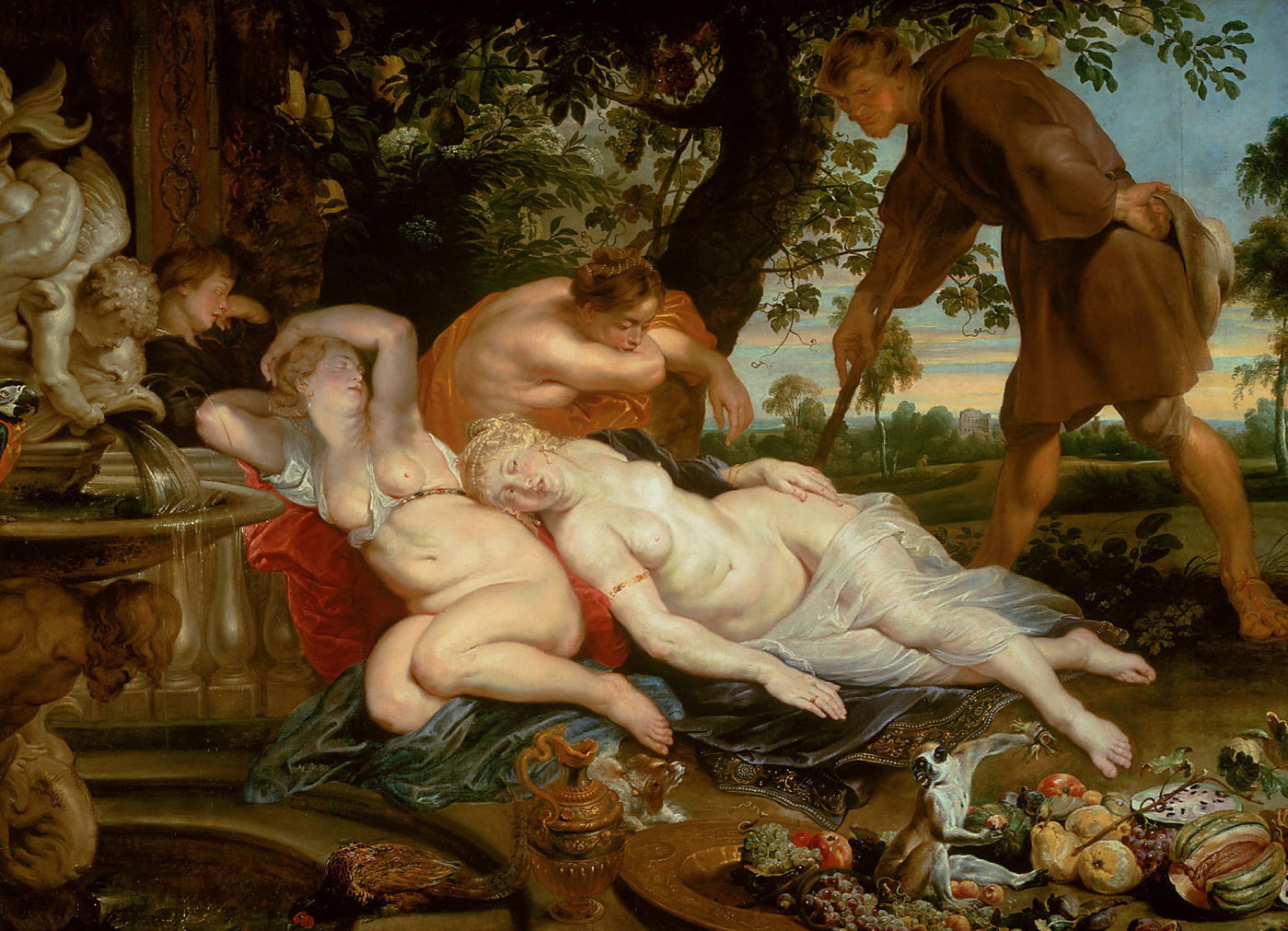
On the fifth day of the Decameron’s stories, Fiammetta chose the theme of the adventures of lovers who survived calamities or misfortunes and reached a state of happiness. The first of those concerns Cimon (or Cymon) and Iphigenia, and was told by Panfilo. This has been painted more than any other story in the whole of the Decameron, by masters from Rubens to Frederic, Lord Leighton, none of whom attempts to tell any more than its opening. Also note that Iphigenia here isn’t the daughter of Agamemnon who had to be sacrificed to bring favourable winds for the Greek fleet to sail against Troy.
Cimon’s father was a wealthy Cypriot, but Cimon, a nickname given in honour of his apparent simplicity and uncouthness, was his problem child. He was exceedingly handsome and had a fine physique, but behaved like a complete imbecile. He appeared unable to learn anything, even basic manners, so was sent to live with the farm-workers on his father’s large estates.
One afternoon in May, Cimon was out walking when he reached a fountain in a clearing surrounded by tall trees. Lying asleep on the grass by that fountain was a beautiful young woman, Iphigenia, wearing a flimsy dress that left nothing to the imagination. Sleeping by her were attendants, two women and a man. Cimon was immediately enraptured, leaned on his stick, and stared at her. As he did so, his simple mind started to change.
Master of the Campana Panels (dates not known), Cymon and Iphigenia (c 1525), tempera on panel, 58 x 170 cm, location not known. Wikimedia Commons.
As with many of Boccaccio’s stories, this is shown on a wedding cassone, here from about 1525. It’s relatively simple: there’s no sign of the attendants, but there is a second image of Cimon walking along a path at the far right.
Peter Paul Rubens (1577–1640), Frans Snyders (1579–1657) and Jan Wildens (1584/86–1653), Cymon and Iphigenia (c 1617), oil on canvas, 208 × 282 cm, Kunsthistorisches Museum, Vienna, Austria. Wikimedia Commons.
In about 1617, Peter Paul Rubens joined with Frans Snyders (who painted the still life with monkeys at the lower right) and Jan Wildens (who painted the landscape background) in their marvellous Cymon and Iphigenia. This is accurate in its details too, with the correct quota of attendants, and a splendid fountain at the left. Cimon really looks like Boccaccio’s uncouth simpleton.
Willem Van Mieris (1662-1747), Cymon and Iphigenia (1698), oil on canvas, 27 x 34.8 cm, Museo Poldi Pezzoli, Milan, Italy. Wikimedia Commons.
Willem Van Mieris’ Cymon and Iphigenia from 1698 treats the scene more in the vein of Poussin or Claude, and again remains faithful to Boccaccio’s details.
Benjamin West (1738–1820), Cymon and Iphigenia (c 1766), oil on panel, 61.3 × 82.6 cm, Yale Center for British Art, New Haven, CT. Wikimedia Commons.
Benjamin West was more coy in both of his depictions of this scene. His earlier Cymon and Iphigenia from about 1766 (above) was well-received at the time. Six years later, in 1773, he reversed the composition, and was even more restrained in the display of flesh, as shown below.
Benjamin West (1738–1820), Cymon and Iphigenia (1773), oil on canvas, 127 x 160.3 cm, Los Angeles County Museum of Art (LACMA), Los Angeles, CA. Wikimedia Commons.Angelica Kauffman (1741–1807), Cymon and Iphigenia (c 1780), oil on canvas, diam 62.2 cm, Gibbes Museum of Art, Charleston, SC. Wikimedia Commons.
A few years later, in about 1780, Angelica Kauffman painted this delightful tondo of Cymon and Iphigenia, another variation on the same theme. The cultural contrast between the young man and woman is not so stark.
John Everett Millais (1829–1896), Cymon and Iphigenia (1848), oil on canvas, dimensions not known, Lady Lever Art Gallery, Liverpool, England. Wikimedia Commons.
When he was only eighteen, John Everett Millais painted what was to be his last work before he embraced Pre-Raphaelite style: Cymon and Iphigenia (1848). At first sight this bears little resemblance to Boccaccio’s story, which is to be expected, as Millais didn’t use the Decameron as his literary reference, but a later re-telling by the English poet John Dryden, to which this is more faithful.
Frederic, Lord Leighton (1830-1896), Cymon and Iphigenia (study) (1884), oil on canvas, 43.1 x 66.2 cm, Art Gallery of New South Wales, Sydney, Australia. Wikimedia Commons.
In 1884, Frederic, Lord Leighton painted what must be the most luxuriant and sensuous version of this scene. This study shows Leighton confirming his composition and use of colour.
Frederic, Lord Leighton (1830-1896), Cymon and Iphigenia (1884), oil on canvas, 218.4 x 390 cm, Art Gallery of New South Wales, Sydney, Australia. Wikimedia Commons.
The finished painting, Cymon and Iphigenia from 1884, shows Iphigenia stretched out languidly in her sleep, in the warmth of the last light of the day; behind her the full moon is just starting to rise. Leighton has changed the season to autumn, with the leaves already brown but the days still hot. Cymon stands in shadow on the right, idly scratching his left knee, gazing intently at Iphigenia.
The story that follows those painted idylls is very different.
When Iphigenia finally awoke, she was surprised to see Cimon there, and recognised him immediately. He insisted on accompanying her to her house, then went to his family home, where he turned a new leaf, and over the following four years transformed himself into the best-dressed, most cultured and refined young man on Cyprus. Despite this transformation, Cimon was unable to persuade Iphigenia’s father to allow him to marry the young woman, but was told she was betrothed to a noble on the island of Rhodes.
When the time came for her marriage, Cimon took an armed vessel and gave chase to the ship carrying Iphigenia to Rhodes. He boarded her ship and abducted her.
With Iphigenia on board, Cimon headed for the island of Crete, where he and his crew had relatives and friends. But shortly after they had altered course, a storm blew up, so violent that it threatened to sink the ship. Unable to tell where they were heading, they ended up taking shelter off the coast of Rhodes, where they were caught up by the ship from which they had just abducted Iphigenia.
When their vessel ran aground, Cimon and his crew were forced ashore, where they were quickly rounded up and thrown into prison, and Iphigenia was returned to her family ready for her wedding. Iphigenia’s fiancé implored the chief magistrate of Rhodes, Lysimachus, to put Cimon to death, but he was held in custody with the rest of his crew.
It happened that Lysimachus was deeply in love with a young woman of Rhodes, who was betrothed to Iphigenia’s future brother-in-law. To Lysimachus’ relief, that marriage had been postponed several times, but it was then decided to hold both weddings in the same ceremony. Lysimachus was aggrieved by this, and decided the only way he could marry the Rhodian woman that he loved was to abduct her. In order to do so, he needed the help of Cimon and his crew, who would undoubtedly be delighted to be able to abduct Iphigenia again.
Lysimachus offered Cimon a deal whereby they would together make off with their partners from the scene of the joint wedding, and they agreed to proceed with that.
Two days later, at dusk, as the weddings were just getting under way, Lysimachus, Cimon and his crew entered the house of the two bridegrooms and seized their brides. Unfortunately, it turned out that both grooms were armed and mounted a determined resistance. Cimon killed Iphigenia’s fiancé with a single blow to the head, and the other woman’s intended husband fell dead following a blow by Lysimachus.
Lysimachus, Cimon, their crew and the two abducted brides then fled to a ship which they sailed to exile in Crete, where the two couples were married, amid great and joyous celebrations. In time, the people of Cyprus and Rhodes forgave them for the violent way they had stolen their brides; Lysimachus and his wife were able to return to Rhodes, and Cimon and Iphigenia returned to live happily ever after on Cyprus.
Sadly, none of the masters who had painted Cimon and Iphigenia seems to have been tempted to depict any of the rest of Panfilo’s story.
I hope that you enjoyed Saturday’s Mac Riddles, episode 338. Here are my solutions to them.
1: The first macOS from the mountains around Tahoe.
Click for a solution
Sierra
The first macOS (10.12 Sierra was the first of the new rebranding) from the mountains (named after the Sierra Nevada) around Tahoe (the mountains around Lake Tahoe).
2: The eighth came from the App Store with Mission Control and a mane.
Click for a solution
Lion
The eighth (MacOS X 10.7 was the eighth major version) came from the App Store (it was originally intended to be available only from the App Store) with Mission Control (introduced in 10.7) and a mane (distinctive of a lion).
3: The sixth came with a time machine and spots.
Click for a solution
Leopard
The sixth (Mac OS X 10.5 was the sixth major version) came with a time machine (it introduced Time Machine) and spots (distinctive of a leopard).
The common factor
Click for a solution
Following each of these came a version with the same name qualified: High Sierra, Mountain Lion and Snow Leopard.
Several of my utilities rely on being able to read log entries from your Mac. For most, this is the only way that you’re ever going to try to access the log. For a few this draws attention to potential problems, when the app discovers it can’t access the log and reports that as an error. This article explains what those errors mean, and what you can do to address them.
Log file layout
Files containing log entries are stored in two main locations in your Mac’s Data volume. The majority of them are in /var/db/diagnostics/, while additional and lengthier log data is stored in files named by UUID in /var/db/uuidtext/.
Those in /var/db/diagnostics/ are grouped into standard folders:
Persist holds tracev3 files that contain regular entries, the most important;
Special has similar files for shorter-life entries;
timesync contains files that enable the entries in tracev3 files to be matched with clock time;
Signpost holds tracev3 files for special entries for measuring performance;
HighVolume is normally empty, but might contain entries during periods when they’re particularly frequent.
Unlike traditional Unix log files, macOS doesn’t keep logs for a fixed period such as five days, but the logd process maintains them constantly to keep their total size within set limits that can’t be altered. Thus the period covered by log entries depends on how frequently entries are written to the log. In extreme cases, that can fall to just a few hours, or could extend to many days, although typically it should be at least 24 hours.
SilentKnight
My most popular app that’s also most frequently run, SilentKnight runs a single check that relies on being able to access the log, to look for XProtect Remediator scan reports.
Each time you run SilentKnight, as it prepares to display its window, it runs four checks on the log, those detailed below for LogUI and XProCheck. If any of those fail, rather than warning you in an alert, it simply disables its check for XProtect Remediator scans, and reports XPR scans not checked. If those pass correctly but it can’t find log entries for the scans, it reports no scans in the last 36 hours instead.
There are complications, though. SilentKnight will only check those scans once a day. If you run it more often than that, it won’t repeat those log checks on the XPR scans, and simply informs you XPR scans not checked. It’s only if you see that for the first check of the day that message suggests there may be a problem with the log. You can also disable checking for XProtect malware scans in the app’s settings.
If you see the message XPR scans not checked when you first run the app, and you haven’t disabled that check, then it’s worth running one of the other log utilities to discover why.
XProCheck, Mints, LogUI
Because these apps are all about inspecting log entries, they incorporate more extensive checks and report errors in more detail. To fetch entries from the log, Mints uses the log show command, while XProCheck and LogUI access them directly through macOS. They all run the following checks when the app is starting up, before its main window is displayed, and will warn you in an alert. When you dismiss that alert, the app will quit to allow you to fix the problem before running it again.
Tests used are:
Is the current user an admin user? If not, the alert below is displayed.
Are there any log files in the Persist folder? If not, report that it can’t find any log files.
Are there any timesync files? If not, report that it can’t find any log timesync files.
Can log show retrieve at least 1 log entry from the last 2 seconds? If it can’t, report that it can’t find any log entries on your Mac.
Mints runs another as well:
Can log show get times in the correct format? If it can’t, report the log time format is incorrect and advise the user to set time to 24-hour format.
Fixes
First, ensure that your Mac isn’t deleting log files in /var/db/diagnostics/ or /var/db/uuidtext/. Some ‘housekeeping’ utilities have taken to doing that, but it saves little space, usually well under 2 GB, and removes a mine of invaluable diagnostic information.
You can get fuller information about what’s in those folders with the Logs button in Mints, which also tells you the date of the oldest log entry. The same information is available in LogUI’s Diagnostics Tool.
The usual recommendation for Macs that aren’t writing any files into the Persist or timesync folders is to perform a clean reinstall of macOS or, for Apple silicon Macs, to restore the Mac in DFU mode. However, you’d be wise to contact Apple Support in the first instance, as this problem has occurred before.
If your log records only go back a few hours, there’s no simple way to reduce the rate at which new entries are written to the log. This article suggests some general approaches, and this article explains how to use custom logging profiles.
In the first of these two articles tracing the history of depictions of the temptation of Saint Anthony, I had reached 1650, when the bizarre composite creatures that flourished in Hieronymus Bosch’s triptych of about 1500-10 were becoming common.
David Teniers the Younger (1610–1690), The Temptation of Saint Anthony (c 1660), media and dimensions not known, Palais des Beaux-Arts, Lille, France. Wikimedia Commons.
The prolific David Teniers the Younger painted several versions of the Temptation of Saint Anthony after about 1650. Most, like this painting now in Lille, show an ordinary landscape with the saint, with the addition of his own species of daemons. Some of these re-use ideas first seen in Bosch’s triptych, such as that of a single figure on the back of a flying narwhal; that figure is wearing an inverted funnel on its head.
David Teniers the Younger (1610–1690), The Temptation of Saint Anthony (c 1650), oil on copper, 55 × 69 cm, Museo Nacional del Prado, Madrid. Wikimedia Commons.
Another of Teniers’ paintings, currently in the Prado, shows three fairly normal humans in a menagerie of daemons, some of which clearly have their origins in Bosch’s work. The figure flying on a fish has changed from the previous painting, but still wears its distinctive inverted funnel.
David Teniers the Younger (1610-1690), The Temptation of Saint Anthony (c 1650), oil on canvas, 80 x 110 cm, National Museum of Western Art, Tokyo. Wikimedia Commons.
This third version, now in Tokyo, repeats many of the same daemons in a different setting, retaining the figure wearing the inverted funnel in close aerial combat.
Domenicus van Wijnen (1661–after 1690), The Temptation of Saint Anthony (c 1685), media and dimensions not known, The National Gallery of Ireland, Dublin. Wikimedia Commons.
Almost two centuries after Bosch’s triptych, more radically different and inventive approaches appear, here in Domenicus van Wijnen’s painting of about 1685. Its daemons are much more human in form, and have proliferated in a way more common in the ‘fairie paintings’ seen around 1840, including some by Richard Dadd. Van Wijnen was a prolific painter of scenes of witchcraft and the ‘dark arts’.
Giovanni Battista Tiepolo (1696–1770), The Temptation of Saint Anthony (c 1740), oil on canvas, 40 x 47 cm, Pinacoteca di Brera, Milan. Wikimedia Commons.
Southern European painters were more likely to keep to more traditional figurative compositions, as used by Tiepolo in about 1740. This is surprising, given the presence of Bosch’s paintings in major collections in both Madrid and Venice.
Henri Fantin-Latour (1836–1904), The Temptation of Saint Anthony (c 1875), oil on canvas, 63.5 x 83.5 cm, National Museum of Western Art, Tokyo. Wikimedia Commons.
Depictions of the Temptation of Saint Anthony remained popular even through the 1800s, although by this time Bosch’s triptych seems to have become long forgotten, and painters seemed no longer to need such excuses to exercise their imagination and inventiveness. The long-awaited publication of Gustave Flaubert’s book The Temptation of Saint Anthony, written in 1874 as a script for a play, brought renewed interest, and a succession of paintings from Henri Fantin-Latour (c 1875, above), Paul Cézanne (c 1875, below), Gustave Moreau (a watercolour), and Fernand Khnopff (1883).
Paul Cézanne (1839–1906), The Temptation of Saint Anthony (c 1875), oil on canvas, 47 x 56 cm, Musée d’Orsay, Paris. Wikimedia Commons.
Cézanne shows the shadowy figure of Saint Anthony slumped against a bush at the left, his arms held out to shield himself from the temptations. The devil is shown in stereotypical form, wearing red robes, with an animal head and horns, behind the saint. In front of them is the naked Queen of Sheba, her right arm held high to accentuate her form. Around her are naked children. In front of Saint Anthony is a black bag presumably containing money, and a book.
Domenico Morelli (1823–1901), The Temptation of Saint Anthony (1878), oil on canvas, 137 × 225 cm, Galleria Nazionale d’Arte Moderna, Rome. Wikimedia Commons.
The influential Neapolitan realist Domenico Morelli painted this stark work in 1878, perhaps the exact antithesis of the rich imagery that had developed since the Renaissance.
Félicien Rops (1833–1898), The Temptation of Saint Anthony (1878), pastel and gouache on paper, 73.8 × 54.3 cm, Cabinet des estampes, Bibliothèque Royale Albert Ier, Brussels. Wikimedia Commons.
That same year, Félicien Rops painted his satirical and irreverent version with more subtle details. Bound to the cross in Saint Anthony’s tempting vision is a visibly voluptuous woman, the word EROS replacing the normal initialism of INRI (Iēsūs/Iēsus Nazarēnus, Rēx Iūdaeōrum, meaning Jesus of Nazareth, the King of the Jews) shown above Christ’s head. Christ himself, with full stigmata, has been knocked sideways to accommodate the woman’s naked body. Behind the cross the horned devil wears scarlet robes and pulls faces. Behind him is a pig, Anthony’s attribute. The two daemonic putti are most definitely not references to Bosch.
Lovis Corinth (1858–1925), The Temptation of Saint Anthony (1897), oil on canvas, 88 × 107 cm, Bayerische Staatsgemäldesammlungen, Munich. Wikimedia Commons.
Lovis Corinth painted two versions of the Temptation. The earlier, from 1897, shows Anthony surrounded by beautiful and naked women, offering him fruit, other food, and their bodies. The daemons have faded into the background, and are caricatures based on humans.
Lovis Corinth (1858–1925), The Temptation of Saint Anthony (after Gustave Flaubert) (1908), oil on canvas, 135.3 × 200.3 cm, The Tate Gallery, London. Wikimedia Commons.
His later canvas, explicitly painted after Gustave Flaubert, in 1908, brings in the Queen of Sheba, an elephant and monkey, but is also notable for depicting Anthony as a young man. Even Salvador Dalí’s 1946 painting of the Temptation steers clear of Bosch’s imagery, although it does at least return to the concept of an individualistic and inventive vision.
I suppose it had to happen that search engines and AI were exploited to deliver malware to the unsuspecting. As that article prompted a brief discussion of the usefulness and reliability of AI-based troubleshooting, I’ve been doing a little checking.
To examine this, I’ve posed Google’s AI some test questions. Rather than run through a long list, I’ve focussed on five that are reasonably frequent but have catches in them. Some are embedded in the question itself, others are inherent in the solution. My aim here isn’t to focus on the strengths of AI, but to understand its weaknesses better, just as you might with a human expert. After all, it doesn’t take much expertise to get the straightforward answers right.
1. How to reduce system data on mac
This question is framed carefully to reveal that the questioner has already used Storage settings, and has been confronted with a great deal of space being used by System Data, an unhelpful category and a situation that’s all too common, as I’ve considered here and elsewhere.
Google’s overview started well, telling me that “System Data includes caches, logs, and temporary files that build up over time and aren’t easily removable like regular documents.” Once it progressed to suggesting actions, though, it repeated a formula it seems to like, but is sadly well out of date: “Use Built-in Storage Management. Click the Apple menu () > About This Mac > Storage > Manage. Use recommendations like ‘Store in iCloud,’ ‘Optimize Storage,’ and ‘Empty Trash Automatically’.” If you try to follow those, you’ll immediately discover that Storage has moved elsewhere. Furthermore, those recommendations won’t tackle the problem framed in the question.
It continues on safer ground, with procedures to clear caches and logs, but those are conducted in Terminal, and there’s no mention of booting in Safe mode. It also directs the user to Terminal to remove snapshots using tmutil rather than Disk Utility. After that, it loses the direction in the question, recommending the user to “remove unused applications and files”, despite the fact that they aren’t included in System Data. Finally, and still off the subject, it mentions using DaisyDisk.
This demonstrates how Google’s AI can’t maintain a logical sequence in troubleshooting, and prefers to direct the user to command tools rather than familiar bundled utilities like Disk Utility, or one of the primary purposes of Safe mode.
2. How to reset home permissions on mac
This has long been a contentious issue, but for the last few years has been fairly settled, as explained here. We no longer reset or repair permissions.
This was Google’s most obvious disaster, as it advised: “To reset home folder permissions on a Mac, boot into Recovery Mode (Command-R), open Terminal, type resetpassword , and use the ‘Reset Home Directory Permissions and ACLs’ button in the utility to fix ownership and permissions for your user account, then restart. For newer macOS versions, Apple also suggests using the repairHomePermissions tool in Recovery, followed by a macOS reinstallation for a full fix, but the resetpassword utility is the primary way to reset the main permissions.”
Of course, Apple silicon Macs don’t use Command-R to enter Recovery Mode, and as you might expect, the resetpassword command opens Recovery Assistant where you can reset your password in the event that you forgot it. That has absolutely nothing to do with permissions, and demonstrates that Google hasn’t understood the question. There’s no such button in that utility, so it’s making things up. It’s also worth nothing that it later recommends that after running repairHomePermissions, you reinstall macOS.
Perhaps the fundamental problem here is the linked support content dating back to 2011, and a failure to recognise how this has changed in the years since. This suggests that its LLM doesn’t take time and change into account, which is deeply concerning when deriving advice on macOS.
3. How to identify clone files in macos
This has been a longstanding problem since the introduction of APFS. Note, though, that question isn’t posed to test whether two or more files are clones of one another, simply how to identify whether files are clones.
Google’s AI Overview is pretty good, and points out that “you need specialized tools or command-line tricks because Finder just sees copies”. However, the next section is titled “Using Finder (for general duplicates)” and gives a facile answer that’s completely inappropriate to that question. This demonstrates how AI always tries to answer, even when it doesn’t know an answer. After that it offers a Terminal solution that again finds duplicates but not clone files, as it doesn’t even check whether the files found have been cloned. It then suggests using specialised apps, including Precize and Sparsity, but lacks useful detail. It ends with pointing out the differences between hard links and clone files, but clearly hasn’t understood a word.
Humans are far more willing to admit they don’t know, and to ask follow-up questions to help them understand exactly what you’re asking.
4. How to run an unsigned app in macos
One of the well-known features of Apple silicon Macs is that, from their first release five years ago, they have only ever run code that has been signed, even if using just an ad-hoc signature, while Intel Macs remain able to run apps and code that has no signature at all. There’s also an important distinction between unsigned code, and code that has been signed by an ad-hoc signature rather than a developer signature.
Those are missed entirely by Google’s AI, as a result of which its answer is riddled with misunderstandings. It recommends what it terms ‘The Standard “Open Anyway”‘ method, which still can’t run unsigned code on Apple silicon. Its final recommendation is to use sudo spctl --master-disable, which disables Gatekeeper and XProtect checks but still doesn’t allow unsigned code to run on Apple silicon.
Given that LLMs are all about language rather than facts or knowledge, it’s surprising that it failed to see the distinction here. This topic was also widely discussed when Apple silicon Macs were introduced, so it’s puzzling that Google was unable to recall any discussion from that time.
5. How to remove com.apple.macl in macos
I’ve only recently revisited this topic, although it dates back to Catalina. This particular extended attribute is frequently added to files, and can have unpleasant consequences when opening or saving them is blocked. Unlike the ordinary quarantine xattr, when macOS applies this one it’s usually protected by SIP, which makes its removal fraught unless you know the trick.
Google AI’s answer made a promising start, writing that “you can use the xattr command in the Terminal, but you might need to use a specific approach depending on your macOS version and file location, as this attribute is often protected by System Integrity Protection (SIP) or file access permissions.” It then ignores the problems posed by SIP protection, and recommends trying the xattr command. As an alternative for “stubborn cases”, it recommends booting into Recovery, and using xattr from there, which should work if you can locate and access the file, which can be quite an achievement in Recovery.
In a bid to remain helpful, it next suggests granting the Terminal app Full Disk Access, although that’s irrelevant. It tries again with: “A common workaround involves moving the file using an application that doesn’t propagate the com.apple.macl attribute, or transferring it to a non-Mac file system.” It finally gets lost when trying to use iCloud Sync.
In common with other answers, Google’s AI started off well, as if it understood the heart of the problem, but quickly demonstrated that it was unable to recall a solution, and stopped making any sense.
Reproducibility
Before you rush off and try the same questions in your favourite AI, a word of warning: the answers you’ll be given will be different from mine, even if you use exactly the same words with Google. This is because randomisation is at the heart of AI, and each time you elicit a response from an LLM, it will differ. Sometimes those differences can be subtle and linguistic, others can manipulate different ‘facts’, or fabricate conflicting answers. This is, apparently, intentional, and hopefully never affects any human expert you consult.
Conclusions
These five questions have demonstrated that Google’s AI can produce some surprisingly accurate information that appears insightful and can match human expertise. In some cases, recommended solutions are sound and well-explained, but in others they appear based on outdated information that may conflict with the opening Overview. Where there aren’t readymade solutions it can quote, it will always try to be helpful in providing an answer, no matter how illogical or flawed that might be. In some cases those could lead an unsuspecting user into danger, and often ignore what was seeded in the original question.
The only way to use Google AI safely is to double-check everything carefully with authoritative sources before trying any of its suggestions, which surely removes much or all of its value.
Paintings of scenes from the hagiographies of Christian saints have been enduring favourites, particularly for churches dedicated to that saint, and for sponsors named after them. The lives of some saints are sufficiently complicated as to offer the artist a choice of different scenes, but in the case of Saint Anthony the Great (of Egypt, the Abbot, etc.), paintings are almost confined to his temptation by the devil.
Saint Anthony was born in 251 CE to wealthy parents in Lower Egypt. His parents died when he was 18. He then became an evangelical Christian, and gave his inheritance away to follow an ascetic life. For fifteen years he lived as a hermit. During this time the devil fought with him, afflicting him with boredom, laziness, and dreams of lustful women, before beating him unconscious.
Friends found him and brought him back to health, so he returned to the desert for another twenty years. This time the devil afflicted him with visions of wild beasts, snakes and scorpions, but again he fought back, eventually emerging serene and healthy. He went to Alexandria during the persecution of Christians there, to comfort those in prison. He returned to the desert, where he built a monastic system with his followers.
His attributes are a bell, a pig, a book, the Tau cross (like a capital T), sometimes with a bell pendant. He is commonly shown being tempted in a wilderness, often by naked women, and is associated with fire (“Saint Anthony’s Fire”).
The visionary nature of his temptation, and the temptations offered him, give a painter a wonderful opportunity to exercise their imagination, and to include content that might otherwise be excluded from places of worship. This weekend I show a selection of paintings of this unique story. This article covers paintings before 1650, and the next will cover the period from 1660 to the early twentieth century.
Stefano di Giovanni (1392–1450), St Antony Beaten by the Devils (1430-32), media and dimensions not known, Pinacoteca Nazionale di Siena, Siena, Italy. Wikimedia Commons.
Painted in 1430-32, Stefano di Giovanni’s St Antony Beaten by the Devils identifies the saint by his Tau crucifix. Three devils, clearly fallen angels by their wings, are beating him with clubs. Those devils are fairly conventional figures, part animal and part man, with horns.
Michelangelo (1475–1564), The Torment of Saint Anthony (c 1487–88), tempera and oil on panel, 47 x 34.9 cm, Kimbell Art Museum, Fort Worth, TX. Wikimedia Commons.
Michelangelo’s The Torment of Saint Anthony (c 1487–88) continues the theme. Saint Anthony is now being held aloft by ten or so devils, including a weird fish with many spines and a trunk-like snout. The devil at the lower left of the group has breasts and a face in its perineum, which almost makes it double-ended.
We then reach a watershed in the unique paintings of Hieronymus Bosch. Records make it clear that he painted several different versions of the Temptation of Saint Anthony, of which it appears that the Lisbon triptych from about 1500-10 is the sole complete survivor, and there’s also the remains of another in a fragment in Kansas City.
Hieronymus Bosch (c 1450–1516), The Temptation of Saint Anthony (Lisbon) (c 1500-10), oil on oak panel, left wing 144.8 x 66.5 cm, central panel 145.1 × 132.8 cm, right wing 144.8 × 66.7 cm, Museu Nacional de Arte Antiga, Lisbon. Wikimedia Commons.
Inside the triptych now in Lisbon, the left panel shows Saint Anthony being assisted by three others, as he crosses a small wooden bridge, in a state of complete exhaustion, perhaps after being beaten unconscious by the devil. In the countryside around that group are weird human and portmanteau animal figures. In the sky above, Saint Anthony is seen again, being flown around on the back of another invented animal.
The centre panel shows Saint Anthony in the middle, kneeling in prayer and surrounded by bizarre figures, creatures, and objects, as if in a vision of temptation. In the background a town is burning.
The foreground shows more scenes involving bizarre figures, creatures, and objects. At the left, a jumble of them emerges from the huge shell of a strawberry-like fruit. One of those figures is astride a goose, and playing a harp. In the middle is a small pond, in which a hybrid between a fish and a boat is floating, and a man is seen inside another strange creature.
The right panel shows Saint Anthony seated, with a book open in front of him. He is again surrounded by strange figures and creatures from a vision of temptation. The background shows a prominent windmill and towers, behind which is a wintry landscape with snow on the ground.
In the foreground, in front of the saint, is a circular table, half-covered with a white tablecloth. The table is supported by naked human figures, one of whom has his left foot in a large pot. Another wears an armoured glove brandishing a heavy scimitar, but a creature has passed a thin-bladed sword through its neck. At the left edge of the table, another naked human is blowing a curiously curved trumpet. To the right an abdomen with ears and legs, wrapped in a red cloth hat, has a sword stuck into it.
Matthias Grünewald (1470-1528), Visit of St Anthony to St Paul and Temptation of St Anthony (c 1515), oil on panel, each panel 265 x 141 cm, Musée Unterlinden, Colmar, France. Wikimedia Commons.
Matthias Grünewald’s slightly later diptych provides useful contrast between the conventional Visit of St Anthony to St Paul on the left, and his Temptation of St Anthony (c 1515) on the right. These daemons are different from Bosch’s, but are nevertheless highly imaginative in their appearance.
Niklaus Manuel (1484–1530), The Temptation of Saint Anthony (Antonius altar, left wing outside: Demons Tormenting St. Anthony) (1520), oil on panel, width 135 cm, Kunstmuseum Bern, Bern, Switzerland. Wikimedia Commons.
The outside of the left panel of Niklaus Manuel’s Antonius altar shows Demons Tormenting St. Anthony (1520). Its daemons, and the wooden clubs with which they attack the saint, are inventive, but still rooted in Stefano di Giovanni’s of a century before.
Lucas van Leyden (1494–1533), The Temptation of Saint Anthony (c 1530), oil on panel, 66 x 71 cm, Koninklijke Musea voor Schone Kunsten van België, Brussels. Wikimedia Commons.
Lucas van Leyden’s painting of about 1530 appears to have been directly influenced by Bosch. Leading its small procession of strange creatures is a man with a bird’s head, and a long bill, wearing ice-skates, clearly derived from the creature bearing a note in the foreground of the left wing of Bosch’s triptych. There are several other familiar features in those creatures, but the rest of the painting is more conventional.
Cornelis Massijs (c 1510/1511–1556/1557), The Temptation of Saint Anthony (c 1540), oil on canvas, Koninklijke Musea voor Schone Kunsten van België, Brussels. Wikimedia Commons.
By about 1540, Cornelis Massijs was still content to paint an almost completely realist image, showing Saint Anthony with two naked women, and another who may be their procuress. But once again there are some small decorations – a pot-bellied man, a creature with an inverted funnel on its head, and a little group at the right – that seem to have invaded from the mind of Bosch.
Pieter Coecke van Aelst (1502–1550), The Temptation of Saint Anthony (1543-1550), oil on panel, 41 x 53 cm, Museo Nacional del Prado, Madrid. Wikimedia Commons.
When we reach Pieter Coecke van Aelst in 1543-1550, the emphasis has changed completely. There are still three normal human figures, of the saint, a tempting nude, and her procuress behind, but the rest of the painting is filled with Bosch derivatives, such as the nun with wings biting someone’s leg, in the foreground. The burning town also makes an appearance in the left distance.
Paolo Veronese (1528–1588), The Temptation of Saint Anthony (1552-3), oil on canvas, 198 x 151 cm, Musée des Beaux-Arts, Caen, France. Wikimedia Commons.
Paolo Veronese’s interpretation from 1552-53 is difficult to read, but the saint is almost completely obscured under a well-muscled devil and a woman whose left breast is exposed. Anthony is sprawled on his back, in his brown habit, his left hand fending off the woman’s hand, his right clutching a book. The devil is holding him down with his left hand, and about to strike him with a club held in his right.
Pieter Huys (c 1519–1584), The Temptation of Saint Anthony (1577), color on wood, 76 × 94 cm, Museum Mayer van den Bergh, Antwerp. Wikimedia Commons.
Pieter Huys’s painting of 1577 is more obviously a derivative from Bosch. Saint Anthony could almost have been copied from one of the earlier paintings, and most of the strange figures and creatures have been borrowed and re-interpreted. Musical instruments such as the lute and harp make an appearance, but many of the symbols have been changed. For example, where Bosch’s triptych features round tables with a white cloth, Huys opts for a rectangular table, and the background has a town burning even more violently.
Maerten de Vos (1532–1603), The Temptation of Saint Anthony (1591-4), oil on panel, 280 x 212 cm, Koninklijk Museum voor Schone Kunsten, Antwerp, Belgium. Wikimedia Commons.
Maerten de Vos’s vision of 1591-4 follows a more traditional line again, although it contains some strange elements that appear more personal. He shows one Saint Anthony apparently carrying another, unconscious Saint Anthony in his arms, rather than the saint supported by friends. There’s a third version of the saint flying in the air, surrounded by daemons, too. That unconscious saint points to a pig, a recognised attribute, but nearby is a pair of lions. One of the more Bosch-like creatures in the right foreground is a portmanteau of human and bird, wears an inverted funnel on its head, and is reading sheet music.
Jan Brueghel the Elder (1568–1625), The Temptation of Saint Anthony (c 1610), oil on canvas, 148 x 230 cm, Museo Nacional de San Gregorio, Valladolid, Spain. Wikimedia Commons.
Just a century after Bosch painted his triptych, Jan Brueghel the Elder combines a cavalcade of more traditional figures with a foreground of more bizarre ones derived from Bosch, including an old person’s head with four human legs, and a bird with two heads, one of a cockerel and the other a duck with a clarinet-like bill. A second image of the saint appears in the sky, surrounded by daemons, and a church is on fire in the background.
Joos van Craesbeeck (c 1605–1654/1661), The Temptation of Saint Anthony (c 1650), oil on canvas, 78 x 116 cm, Staatliche Kunsthalle, Karlsruhe, Germany. Wikimedia Commons.
By about 1650, Joos van Craesbeeck was using some of Bosch’s iconography with his own developments. The use of a human head as a container is probably derived from Bosch’s tree-man and similar devices, but here has become even more realistic. To the right of that, a naked man sits facing backwards on a duck-horse: he is playing a stringed musical instrument, and wearing an inverted funnel on his head. Van Craesbeeck’s humans seem to have grown small red tails too. Oddly, van Craesbeeck doesn’t place the Greek letter Tau on the saint’s robes, but the Roman letter A, perhaps monogrammed with Tau. That appears unique to this painting.
macOS apps manage the contents of their own windows, drawing and refreshing them as needed. To assemble all those into what you see on the display requires the services of the master compositor, WindowServer. From the moment the login window appears during startup, WindowServer is hard at work, and remains so until you shut your Mac down. Without WindowServer there could be no GUI.
Open Activity Monitor, and you’ll see WindowServer close to the top of the lists of CPU, Memory and Energy users, and when it’s getting into trouble that’s always a good place to check what’s going on. You may also notice that it’s one of a pair of processes including distnoted with their own user, _windowserver. They’re part of a group of interconnected services that handle window management, compositing of windows into the display image, and event-routing for apps, with distnoted responsible for system message notification. In the log, WindowServer is often associated with the com.apple.SkyLight subsystem.
Compositing
You can get a good idea of what WindowServer does using screenshots. Using Command-Shift-4, then pressing the Space Bar and selecting a window, you’ll get a shot of an individual window, as shown in the examples below.
WindowServer then positions them according to their current locations on the whole display, and produces a layered composite, as you’ll see in a screenshot taken with Command-Shift-3.
That composite is then sent through the graphics driver to graphics output hardware.
With its central position in managing windows and compositing them, WindowServer is also responsible for handling Spaces (introduced in Mac OS X 10.5 Leopard), window tabs, multiple displays, and behaviours that stream or extract parts or all of a display image, such as taking screenshots. Because WindowServer knows which app’s windows are where, and which are at the front, it also routes events to each app. For example, when you click on a window it’s WindowServer that determines which app owns it, and passes the event to that app to handle.
Increasing demands
This has become more involved since the introduction of Catalyst apps from macOS 10.14 to 11, and more so since Apple silicon Macs have brought the ability to run iOS and iPadOS apps. iOS uses a series of -board services in its GUI, including SpringBoard as the Home Screen manager instead of the Finder, FrontBoard to manage the app’s scenes, and FuseBoard its menus, which are now run in macOS as well. RunningBoard, which manages the resources available to apps and processes, has been incorporated into macOS for some years.
The introduction of Stage Manager in macOS Ventura in 2022 has also been stretching WindowServer, and can substantially increase its demands on CPU and memory.
Troubleshooting
You can reduce WindowServer’s workload by closing tabs and windows, turning Stage Manager off, reducing the number of Spaces, and quitting non-essential apps. Even when window or tab contents aren’t visible, they still have to be managed.
If WindowServer stops working, for instance when it crashes, not only does everything on the display(s) freeze, but routing of input events such as clicks or taps also stops. Although in the past macOS has sometimes been able to log the current user out and restart WindowServer, fatal WindowServer problems are now most likely to result in a kernel panic or a complete freeze. If your Mac freezes rather than restarts, a forced shutdown may be your only way forward. Recurrent WindowServer crashes suggest a problem with the graphics driver or graphics hardware, and should always be reported to Apple via Feedback.
Summary
WindowServer works between app window management and display drivers to composite windows and on-screen items, producing the image to be displayed.
With distnoted it also routes events to apps, and manages system message notification.
Demands on its services are increased with Spaces and Stage Manager, and it works with the different expectations of Catalyst and iOS/iPadOS apps running in macOS.
When it fails, displays freeze and input responses cease. If those don’t precipitate a kernel panic and restart, a forced shutdown may be the only solution.
The update from macOS Tahoe 26.1 to 26.2 is fairly large, but appears to be largely routine maintenance, together with some important security updates.
At last, Apple has provided more detail of some of the improvements and changes in this summary. These include a new Edge Light feature to light your face during low-light video calls, Podcasts gaining automatic chapter generation, filters added to the Games library, AirDrop codes providing an additional means of verification with unknown contacts, and enhancements to Freeform tables.
Security release notes report a total of 46 vulnerabilities addressed. Among those are multiple WebKit vulnerabilities, including two that Apple believes have been exploited already “in an extremely sophisticated attack against specific targeted individuals” in earlier versions of iOS. Those alone make 26.2 a compelling early update.
The build number of macOS 26.2 is 25C56, it updates iBoot firmware to version 13822.61.10 on Apple silicon Macs and Intel firmware to 2094.40.1.0.0 (iBridge 23.16.12048.0.0,0). Note that Intel Macs only have an update to iBridge, and not their EFI firmware this time.
Significant changes seen in bundled apps include:
Freeform, to version 4.2
Music, to version 1.6.2
Passwords, to version 2.2
Safari, to version 26.2 (21623.1.14.11.9)
TV, to version 1.6.2.
Significant changes seen in /System/Library are relatively few, with many minor increments to build numbers. Notable changes include:
All AGX kernel extensions are updated
AppleDockConnect is a new kernel extension to accompany AppleDockChannel
AppleThunderboltRDMA is another new kernel extension
APFS is updated to version 2632.40.17, a tiny increment
the webcontentfilter kext has been removed
there is no change in the RichText.mdimporter for Spotlight indexing, implying that no bugs have been fixed in it.
The total number of bundles in that folder has only increased slightly, from 9785 to 9832.
One common criticism of the new Liquid Glass option added to Appearance settings in 26.1 is that Reduce transparency in Accessibility settings no longer reduces some transparency effects. There has been no change in that behaviour in 26.2, which continues to apply Liquid Glass effects in locations such as sidebars despite Reduce transparency being turned on. Our cries have clearly fallen on deaf ears.
I have also confirmed, as I suspected from the lack of change in the RichText.mdimporter, that the ‘LG bug’ in Spotlight remains, and still hasn’t been fixed.
Apple has just released the update to bring macOS Tahoe to version 26.2, and security updates to Sequoia and Sonoma to bring them to 15.7.3 and 14.8.3 respectively. The latter two should also have associated Safari updates.
The update to 26.2 is about 3.78 GB to download to an Apple silicon Mac, and 2.5 GB for an Intel Mac. Some Macs may require larger downloads, though, with some in excess of 10 GB.
Tahoe 26.2 introduces Edge Light to light your face during low-light video calls, improves Podcasts with automatic chapter generation, adds filters to the Games library, adds AirDrop codes as an additional verification with unknown contacts, enhances Freeform tables, and more. Fuller release notes are available here, and are a significant improvement in themselves.
Security release notes for Tahoe report a total of 46 vulnerabilities addressed. Among them are multiple WebKit vulnerabilities, including two that Apple believes have been exploited already “in an extremely sophisticated attack against specific targeted individuals” in earlier versions of iOS. Notes for Sequoia list 25, and those for Sonoma 21. The Safari update for Sequoia and Sonoma does address those critical vulnerabilities.
Its macOS build number is 25C56, it updates iBoot firmware to version 13822.61.10 on Apple silicon Macs and Intel firmware to 2094.40.1.0.0 (iBridge 23.16.12048.0.0,0), and brings Safari to version 26.2 (21623.1.14.11.9).
During the first few years of the twentieth century, the former Nabi painter and print-maker Félix Vallotton had concentrated on painting mysterious interiors, as well as portraits and other figurative works.
Félix Vallotton (1865–1925), Le Bain turc (The Turkish Bath) (1907), oil on canvas, 30.5 x 195.5 cm, Les Musées d’art et d’histoire de Genève, Geneva, Switzerland. Wikimedia Commons.
By 1907, when he painted this Orientalist Turkish Bath, his figures had become modern in appearance. With their tied-up hair, it would be easy to mistake this as a painting from fifty years later.
Félix Vallotton (1865–1925), Andromeda Standing with Perseus (1907), oil on canvas, 92 x 73 cm, Private collection. Wikimedia Commons.
That same year, he started painting scenes from classical myth, here Andromeda Standing with Perseus (1907). This shows the sea monster Cetus heading for a defenceless Andromeda, as hero Perseus charges to her aid through a cleft in the black sky. He has lost his classical attribute of the head of Medusa, and here rides the winged horse Pegasus while holding a knight’s lance. The horse’s wings form an edge to the black sky as it carves through the air. Each figure is colour coded: green for the sea monster, pink for the near-victim, and blue for the hero, against a straw-coloured sea.
Félix Vallotton (1865–1925), The Rape of Europa (1908), oil on canvas, 130 x 162 cm, Kunstmuseum Bern, Bern, Switzerland. Wikimedia Commons.
The following year, he again broke with convention in his painting of The Rape of Europa (1908). In this clean and simplified account, we look out to sea as the naked Europa clambers onto the back of Jupiter disguised as a brown bull. Given the long-established literary and artistic tradition of the bull being white, this can only have been a deliberate choice on his part.
Félix Vallotton (1865–1925), La Mare, Honfleur (The Pond) (1909), media and dimensions not known, Kunstmuseum Basel, Basel, Switzerland. Wikimedia Commons.
In addition to mythological narratives, Vallotton started painting more landscapes, some of which are unusual and innovative, like La Mare, Honfleur (1909), showing a pond at night near the north coastal town of Honfleur. The black plane of the water has ripples travelling from a point at the right edge. In the left foreground is a stand of long grass and weeds bowed over in an arc, and behind the blossom on a tree glows in the dark.
Félix Edouard Vallotton (1865-1925), Perseus Killing the Dragon (1910), oil on canvas, 160 x 233 cm, Musée d’art et d’histoire de Genève, Geneva. By Codex, via Wikimedia Commons.
Vallotton returned to the story of Perseus and Andromeda in 1910, in his Perseus Killing the Dragon, which is no sequel to his earlier work. Here he catches the height of peripateia and action, as Perseus is slaying Cetus. Andromeda, long freed from her chains, squats, her back towards the action, at the far left. Her face shows a grimace of slightly anxious disgust towards the monster. Perseus is also completely naked, with no sign of winged sandals, helmet of Hades, or any bag containing Medusa’s head. He is braced in a diagonal, his arms reaching up to exert maximum thrust through the shaft of a spear impaling Cetus through the head. The monster is shown as an alligator, its fangs bared from an open mouth.
Félix Vallotton (1865–1925), Coquèterie (Sauciness) (1911), oil on canvas, 89 x 116 cm, Private collection. Wikimedia Commons.
In Sauciness from 1911, we see a young woman still undressed in her white chemise, her unmade bed behind. She looks at herself in the mirror of a small dressing table, wondering what to wear.
Félix Vallotton (1865–1925), Honfleur in Fog (1911), oil on canvas, dimensions not known, Musée des Beaux-Arts, Nancy, France. Image by Ji-Elle, via Wikimedia Commons.
His Honfleur in Fog from 1911 isn’t a conventional view of this small port on the north French coast, as it looks down from Mont-Joli to the west of the town centre. It captures exactly the sort of transient effects that had been the concern of Impressionism, but in Vallotton’s distinctive style.
Félix Vallotton (1865–1925), Night With Light Fog (1913), further details not known. Wikimedia Commons.
In 1913, Vallotton returned to transient atmospheric effects in Night With Light Fog. Influenced by his print-making, he distils this scene into simple geometry, with almost two-thirds of his canvas the vague purple forms of the town and sky, and three simple bands below it. The lone lamppost and figure at the extreme left restore context.
Félix Vallotton (1865–1925), Self-portrait in a Dressing Gown (1914), oil on canvas, 81 x 65 cm, Musée cantonal des beaux-arts, Lausanne, Switzerland. Wikimedia Commons.
He painted this Self-portrait in a Dressing Gown at a turning point in 1914, just as the world was about to enter the Great War, and he was to enter his fifties, the start of the next and final article in this account of his career and art.
The Messages app is a wonderful way to keep in touch with friends and relatives no matter where they are, and share photos and videos. This article tries to answer the seemingly simple question as to where those are stored, and what this has to do with syndication. I’m grateful to Jack for asking.
Sharing in Messages
If you have more than one Mac or Apple device connected to iMessage, and share that via Messages in iCloud, you’ll no doubt have discovered that shared photos and videos sync across them reasonably well. Delete an image on one, and it should be removed on all the others so long as they’re running, awake and can sync with iCloud.
Those shared photos and videos don’t appear in your System Photo Library, though, unless you save them there. That System Photo Library can share its contents using iCloud Photos, Shared Albums and iCloud Shared Photo Library, but those are separate from sharing in Messages. Turn all Photos sharing off and that doesn’t affect those shared in Messages.
Unfortunately, information about those shared images and videos, and control over them, is primitive in macOS compared with iOS. On an iPhone, you can manage storage for Messages in iCloud in much greater detail, and can view those that are taking up most space. That isn’t offered in macOS 26 Tahoe, only the total space used by Messages in iCloud. Nor is there any Photos library or other location obvious on your Mac that appears to store them.
Syndication Photos Library
Jack isn’t the first to discover this, but if you care to look in ~/Library/Photos/Libraries you’ll find a hidden Photos library named Syndication.photoslibrary that has a similar if not identical structure to a regular photoslibrary. If you look inside that, in the path scopes/syndication/originals you’ll see folders numbered with a single hexadecimal digit, and inside those are many of the shared photos and videos from Messages.
Try copying or duplicating Syndication.photoslibrary into your Picture folder, then launch the Photos app with the Option key held so you’re asked to select a Photos library to open. There pick Syndication.photoslibrary and browse its contents. Although that should look similar to the images and videos still stored in your local Messages, you may well notice there are differences, with the Syndication Photos Library containing more, sometimes a great deal more, than Messages.
But there’s more
Checking on my iPhone, Settings there reports that Messages is currently using 523 MB for photos, 14.7 MB for videos, and 1.1 MB for GIFs and Stickers, making a total of just under 540 MB. Yet on my iMac Pro Syndication.photoslibrary is only 394.1 MB, nearly 150 MB smaller, and on my Mac mini M4 Pro it’s a huge 1.14 GB, although each of them should be storing the same photos and videos. Some users have reported Syndication.photoslibrary of huge size, sometimes tens of GB, suggesting that they either never perform housekeeping on shared images and video in Messages, or theirs have accumulated many orphaned items.
Those Syndication Photos Libraries are the location of photos and videos for Messages, though. Try deleting a photo or two in Messages, and you’ll see each of them update in synchrony.
There’s another puzzle too: if you have some older Photos Libraries, look inside them and you may well see photos and videos in folders in the path scopes/syndication/originals, just as you do in Syndication.photoslibrary. This suggests that the separate Syndication Photos Library may have originally been saved in the current System Photo Library rather than in ~/Library/Photos/Libraries/Syndication.photoslibrary.
My last mystery comes from the list of open files provided by Activity Monitor. With both Messages and Photos apps running, guess which has the database inside Syndication.photoslibrary open? No, not Messages, but Photos.
Conclusions
~/Library/Photos/Libraries/Syndication.photoslibrary is the Photos Library now used to store shared photos, videos, GIFs and Stickers for the Messages app.
Although it syncs changes promptly, some local copies appear to accumulate contents that aren’t removed by Messages.
As a result, some Syndication Photos Libraries grow far larger than required, but there’s no way to force them to purge unused contents.
Throughout much of Europe, bread has been a staple food for the whole of recorded history, and has become a symbol of life in both language and visual art.
Jean-François Millet (1814–1875), Ceres (The Summer) (c 1864-65), oil on canvas, Musée des Beaux-Arts, Bordeaux, France. Wikimedia Commons.
For the classical civilisations of the Mediterranean, this was embodied in the goddess of Jean-François Millet’s Ceres (The Summer) from about 1864-65. She stands, her breasts swollen and ready for lactation, her hair adorned with ripe ears of wheat, a sickle in her right hand to cut the harvest, and a traditional winnow to separate grain from chaff in her left hand. At her feet is a basketful of bread, with ground flour and cut sheaves of wheat behind. The background shows the wheat harvest in full swing, right back to a group of grain- or hay-stacks and an attendant wagon in the distance.
Bread and its sharing is one of the central symbols of Christian beliefs, most notably in the Last Supper, the meal shared by Christ with his disciples before his crucifixion.
Giampietrino (1495–1549), copy after Leonardo da Vinci (1452–1519), The Last Supper (c 1520), oil on canvas, 298 x 770 cm, The Royal Academy of Arts, London. Wikimedia Commons.
The most famous painting of The Last Supper, and one of the best-known works in the European canon, is of course Leonardo da Vinci’s. Giampietrino’s copy from about 1520 gives the closest impression today of what the original must have looked like. Even this copy has been horribly mutilated: the upper third was cut off, and its width reduced, but at least what remains gives a better idea of the original’s appearance.
Leonardo’s composition wasn’t entirely revolutionary for the time. Previous paintings of The Last Supper had spread the apostles along the length of a table, with Christ at its centre. However, Judas Iscariot was usually placed alone on the near side, his back to the viewer, and sometimes with his bag of silver visible behind his back.
Leonardo shows the moment of surprise and denial when Christ announces that one of those sat around the table would betray him. In this, he was perhaps the first artist to assemble the apostles into small groups, a feature that has been repeated in innumerable images following this. Arrayed along the front of the table is a series of round bread rolls and small glasses of red wine.
Paolo Veronese (1528–1588), The Supper at Emmaus (c 1559), oil on canvas, 241 × 415 cm, Musée du Louvre, Paris. Wikimedia Commons.
After his crucifixion and resurrection, Christ appeared several times to his disciples. In The Supper at Emmaus, painted here by Paolo Veronese, two disciples had travelled on the road from Jerusalem to Emmaus as pilgrims, and recognised Christ as he “sat at meat with them, he took bread, and blessed it, and brake, and gave it to them.”
The painting contains separate passages to cue this narrative: on the far left is an asynchronous ‘flashback’ referring to the journey to Emmaus. Christ is in the centre of the painting, identified by his halo, and in the midst of breaking bread. With him at the table are the two bearded figures of the disciples, dressed as pilgrims and bearing staves. On Christ’s right is a servant, acting as waiter to the group. The onlookers dressed in contemporary costume are an aristocratic Italian family of the day, whose portraits are combined.
Christian rites reiterate the Last Supper in Eucharist, and the blessing of bread plays other roles in its religious ceremonies.
Mykola Pymonenko (1862–1912), Waiting for the Blessing (1891), oil on canvas, 133 x 193 cm, Rybinsk Museum-Preserve Рыбинский историко-архитектурный и художественный музей-заповедник, Rybinsk, Russia. Wikimedia Commons.
Mykola Pymonenko’s Waiting for the Blessing (1891) shows the scene at a country church in Ukraine at dawn on Easter Sunday. The local population is crowding inside, while the women gather with their Paska, traditional ornamental bread that must be blessed before it can be eaten as a brunch.
Bread appears elsewhere as a symbol of life, particularly in the context of poverty and charity.
Edmund Blair Leighton (1852–1922), The Charity of Saint Elizabeth of Hungary (c 1895), oil on panel, 26.7 x 20.3 cm, location not known. Wikimedia Commons.
Edmund Blair Leighton’s Charity of Saint Elizabeth of Hungary from about 1895 shows a famous woman who built a hospital where she personally served the sick. Born in 1207, she died in 1231 at the age of only twenty-four. Leighton doesn’t show her in a nursing role, though, but handing out loaves to feed the poor.
Elizabeth Nourse (1859–1938), The Family Meal (1891), engraving from Charles M. Kurtz, ‘Illustrations from the Art Gallery of the World’s Columbian Exposition’, Philadelphia, 1893, further details not known. Wikimedia Commons.
Elizabeth Nourse painted some social realist works looking at the lives of the rural poor. Among these is The Family Meal from 1891, which was awarded a medal at the World’s Columbian Exposition in Chicago in 1893, and is seen here as an engraving in its catalogue. Parents sit with their two young children at an almost bare table. Their meal consists of a pot of soup and the remains of a loaf of what appears to be stale bread. The older child looks expectantly at her mother, who stares despondently at the table. Her husband stares down at his empty bowl.
Philip Hermogenes Calderon (1833–1898), “Lord, Thy Will Be Done” (1855), oil on canvas, 55.9 x 46.4 cm, The Yale Center for British Art, New Haven, CT. Wikimedia Commons.
The wonderfully named Philip Hermogenes Calderon painted his “Lord, Thy Will Be Done” in 1855. This quotation is derived from the Gospel account of what became the Lord’s Prayer, and has subsequently been used on many Christian religious occasions.
A young mother cradles her baby on her lap, looking up to the left. She’s living in difficult circumstances, but isn’t destitute, and wears a wedding ring on her left hand. The carpet is badly worn, and the coal scuttle empty, but there’s a loaf of bread on the table: she has her ‘daily bread’, another reference to the Lord’s Prayer. A portrait of a fine young man hangs above the mantlepiece, indicating her husband and the baby’s father is currently absent on military service. Several issues of The Times newspaper are scattered on the floor at the right, as if the woman has been following news of a military campaign overseas. Under the table is a letter, most probably from her husband.
Christian Krohg (1852–1925), The Struggle for Existence (1889), oil on canvas, 300 x 225 cm, Nasjonalgalleriet, Oslo, Norway. Wikimedia Commons.
Christian Krohg’s The Struggle for Existence, also translated as The Struggle for Survival from 1889 shows Karl Johan Street in Oslo in the depths of winter, almost deserted except for a tight-packed crowd of poor women and children queuing for free bread. These people are wrapped up in patched and tatty clothing, clutching baskets and other containers in which to put the food. A disembodied hand is passing a single bread roll out to them, from within the pillars at the left edge. That was yesterday’s bread; now stale, the baker is giving it away only because he cannot sell it.
Google is so helpful now when you ask it to solve a problem, such as how to free up space on your Mac. Not only can it make its own suggestions, but it can tap into those from AIs like ChatGPT and Grok. This article shows how that can bring you malware, thanks to the recent research of Stuart Ashenbrenner and Jonathan Semon at Huntress.
Please don’t try anything you see in this article, unless you want AMOS stealer malware on your Mac.
I started by entering a common search request, clear disk space on macOS, the sort of thing many Mac users might ask.
At the top of Google’s sponsored results is an answer from ChatGPT, giving its trusted web address. When I clicked on that, it took me to ChatGPT, where there’s a nice clear set of instructions, described impeccably just as you’d expect from AI.
This helpfully tells me how to open Terminal using Spotlight, very professional.
It then provides me with a command I can copy with a single click, and paste straight into Terminal. It even explains what that does.
When I press Return, I’m prompted for my password, which I enter.
Although I was a bit surprised to see this prompt, it looks genuine, so I allowed it.
Far from clearing space on my Mac, the malware, an AMOS stealer, has gone to work, saving a copy of the password I gave it, in the /tmp folder, and installing its payload named update.
Scripts like .agent are installed in my Home folder, and my (virtual) Mac is now well and truly owned by its attacker.
As Ashenbrenner and Semon point out, this marks a new and deeply disturbing change, that we’re going to see much more of. We have learned to trust many of the steps that here turn out to lead us into trouble, and there’s precious little that macOS can do to protect us. This exploit relies almost entirely on our human weakness to put trust in what’s inherently dangerous.
First, distrust everything you see in search engines. Assess what they return critically, particularly anything that’s promoted. It’s promoted for a reason, and that’s money, so before you click on any link ask how that’s trying to make money from you. If that’s associated with AI, then be even more suspicious, and disbelieve everything it tells you or offers. Assume that it’s a hallucination (more bluntly, a lie), or has been manipulated to trap you.
Next, check the provenance and authenticity of where that click takes you. In this case, it was to a ChatGPT conversation that had been poisoned to trick you. When you’re looking for advice, look for a URL that’s part of a site you recognise as a reputable Mac specialist. Never follow a shortened link without unshortening it using a utility like Link Unshortener from the App Store, rather than one of the potentially malicious sites that claims to perform that service.
When you think you’ve found a solution, don’t follow it blindly, be critical. Never run any command in Terminal unless it comes from a reputable source that explains it fully, and you have satisfied yourself that you understand exactly what it does. In this case the command provided was obfuscated to hide its true action, and should have rung alarm bells as soon as you saw it. If you were to spare a few moments to read what it contains, you would have seen the command curl, which is commonly used by malware to fetch their payloads without any quarantine xattr being attached to them. Even though the rest of the script had been concealed by base-64 encoding, that stands out.
If you did get as far as running the malicious script, then there was another good clue that it wasn’t up to anything good: it prompted you for a System Password:. The correct prompt should just be Password:, and immediately following that should be a distinctive key character that’s generated by macOS for this purpose. Then as you typed your password in, no characters should appear, whereas this malware showed them in plain text as you entered them, because it was actually running a script to steal your password.
Why can’t macOS protect you from this? Because at each step you have been tricked into bypassing its protections. Terminal isn’t intended to be a place for the innocent to paste obfuscated commands inviting you to surrender your password and download executable code to exploit your Mac. curl isn’t intended to allow malware to arrive without being put into quarantine. And ad hoc signatures aren’t intended to allow that malicious code to be executed.
As I was preparing this article Google search ceased offering the malicious sponsored links, but I expect they’ll be back another time.
AI is certainly transforming our Macs, in this case by luring us to give away our most precious secrets. This isn’t a one-off, and we should expect to see more, and more sophisticated, attacks in the future. Now is the time to replace trust with suspicion, and be determined not to fall victim.
Apple has just released an update to XProtect, bringing it to version 5324. As usual, it doesn’t release information about what security issues this update might add or change.
This version adds another new Yara rule in its TIMELYTURTLE series, for MACOS.TIMELYTURTLE.SWNOA, and amends the recent rules for MACOS.SOMA.AUENB and MACOS.DUBROBBER.CHBI. In the new XPScripts.yr file introduced in XProtect 5322, it reverses the order of the two rules and amends MACOS.OSASCRIPT.COTABR.
You can check whether this update has been installed by opening System Information via About This Mac, and selecting the Installations item under Software.
A full listing of security data file versions is given by SilentKnight and SystHist for El Capitan to Tahoe available from their product page. If your Mac hasn’t yet installed this update, you can force it using SilentKnight or at the command line.
If you want to install this as a named update in SilentKnight, its label is XProtectPlistConfigData_10_15-5324
Sequoia and Tahoe systems only
This update has already been released for Sequoia and Tahoe via iCloud. If you want to check it manually, use the Terminal command sudo xprotect check
then enter your admin password. If that returns version 5324 but your Mac still reports an older version is installed, you should be able to force the update using sudo xprotect update